Difference between revisions of "Screenshots"
(→Project Folders) |
(→Master Regulator Analysis) |
||
| (44 intermediate revisions by 2 users not shown) | |||
| Line 5: | Line 5: | ||
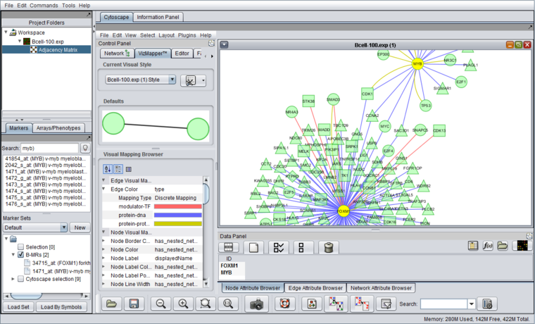
The geWorkbench graphical interface with a CNKB query result dislayed in Cytoscape. | The geWorkbench graphical interface with a CNKB query result dislayed in Cytoscape. | ||
| − | [[Image: | + | [[Image:geWorkbench_Main_Cytoscape_no_frame.png|{{ImageMaxWidth}}]] |
==geWorkbench Configuration== | ==geWorkbench Configuration== | ||
| Line 15: | Line 15: | ||
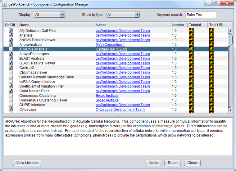
[[Image:CCM_Main.png|{{ImageMaxWidth}}]] | [[Image:CCM_Main.png|{{ImageMaxWidth}}]] | ||
| − | == | + | ==Workspace and Data Management== |
| − | === | + | ===Workspace=== |
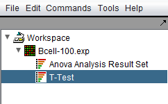
| − | Data sets are loaded into | + | Data sets are loaded into the Workspace. Individual analysis results are stored under their parent dataset. |
| − | [[Image: | + | [[Image:Workspace_with_results.png]] |
===Array/Phenotypes=== | ===Array/Phenotypes=== | ||
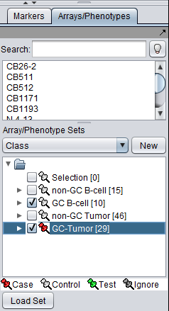
Sets of arrays can be defined and included or excluded from particular analyses (via checkboxes). Sets can be individually marked as belonging to case (here indicated with a red thumbtack) or control groups. | Sets of arrays can be defined and included or excluded from particular analyses (via checkboxes). Sets can be individually marked as belonging to case (here indicated with a red thumbtack) or control groups. | ||
| − | [[Image:T-test_Set_selection_BCell.png | + | [[Image:T-test_Set_selection_BCell.png]] |
===Markers=== | ===Markers=== | ||
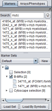
Sets of arrays can be defined and included or excluded from particular analyses (via checkboxes). | Sets of arrays can be defined and included or excluded from particular analyses (via checkboxes). | ||
| − | [[Image:Marker_Sets_Example.png | + | [[Image:Marker_Sets_Example.png]] |
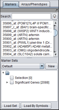
In addition, routines such as ANOVA or t-test return lists of significant markers to the Markers component. | In addition, routines such as ANOVA or t-test return lists of significant markers to the Markers component. | ||
| − | [[Image:ANOVA_Example_Markers.png | + | [[Image:ANOVA_Example_Markers.png]] |
===Retrieval from caArray=== | ===Retrieval from caArray=== | ||
| Line 41: | Line 41: | ||
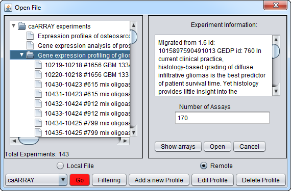
Microarray data can be retrieved directly from instances of caArray. | Microarray data can be retrieved directly from instances of caArray. | ||
| − | [[Image:Open_File_Remote_caArray_show_arrays.png | + | [[Image:Open_File_Remote_caArray_show_arrays.png]] |
== Microarray Data Displays== | == Microarray Data Displays== | ||
| Line 49: | Line 49: | ||
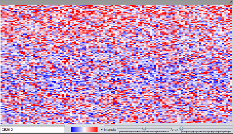
| − | [[Image: | + | [[Image:Microarray_Viewer.png|{{ImageMaxWidth}}]] |
---- | ---- | ||
| Line 57: | Line 57: | ||
| − | [[Image: | + | [[Image:Tabular_Microarray_Viewer.png]] |
---- | ---- | ||
| Line 70: | Line 70: | ||
=== Color Mosaic === | === Color Mosaic === | ||
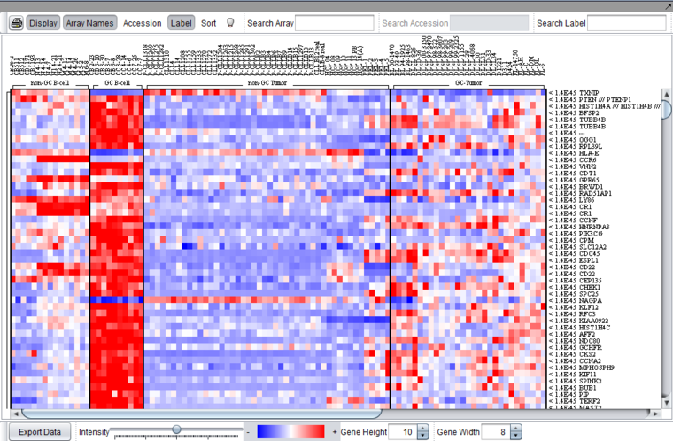
| − | The Color Mosaic component displaying | + | The Color Mosaic component displaying a result from ANOVA analysis. It can also directly display the loaded expression data, or subsets of that data created using Marker and Array sets. |
| − | [[Image: | + | [[Image:Color_Mosaic_ANOVA.png|{{ImageMaxWidth}}]] |
---- | ---- | ||
=== Expression Profile === | === Expression Profile === | ||
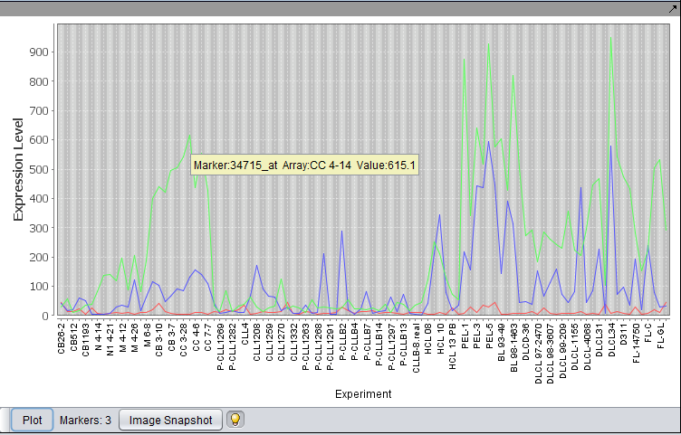
| − | Expression Profile plotting values for selected markers and arrays. | + | Expression Profile plotting values for selected markers and arrays. Individual values can be seen by hovering over a desired data point. |
| − | |||
| − | [[Image: | + | |
| + | [[Image:Expression_Profiles.png|{{ImageMaxWidth}}]] | ||
---- | ---- | ||
| − | |||
===Expression Value Distribution=== | ===Expression Value Distribution=== | ||
| + | The dataset has been quantile normalized and log2 transformed. | ||
| − | [[Image: | + | [[Image:Expression_Value_Distribution.png|{{ImageMaxWidth}}]] |
---- | ---- | ||
| Line 99: | Line 99: | ||
====Array vs Array==== | ====Array vs Array==== | ||
| − | [[Image: | + | [[Image:Scatter_Plot_array_vs_array.png]] |
====Marker vs Marker==== | ====Marker vs Marker==== | ||
| − | [[Image: | + | [[Image:Scatter_Plot_marker_vs_marker.png]] |
---- | ---- | ||
| − | |||
==Gene and Pathway Annotations== | ==Gene and Pathway Annotations== | ||
===Marker Annotations=== | ===Marker Annotations=== | ||
| − | Retrieve and display gene and pathway information from | + | Retrieve and display gene and pathway information from bioDBNet. |
| − | [[Image: | + | [[Image:Marker_Annotations_bioDBNet.png]] |
---- | ---- | ||
| Line 119: | Line 118: | ||
===Marker Annotations - BioCarta Pathways=== | ===Marker Annotations - BioCarta Pathways=== | ||
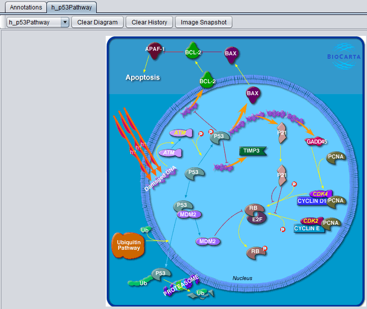
| − | Displays BioCarta images retrieved | + | Displays BioCarta images retrieved via bioDBNet. |
| − | [[Image: | + | [[Image:Marker_Annotations_Pathway_bioDBNet.png|{{ImageMaxWidth}}]] |
| − | |||
| − | |||
| − | |||
| − | |||
| − | |||
| − | |||
| − | |||
| − | |||
---- | ---- | ||
| Line 137: | Line 128: | ||
===Gene Ontology Term Over-representation Analysis=== | ===Gene Ontology Term Over-representation Analysis=== | ||
| − | [[Image: | + | [[Image:GO_Terms_Table_Browser.png|{{ImageMaxWidth}}]] |
===T Test=== | ===T Test=== | ||
| Line 144: | Line 135: | ||
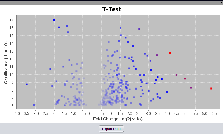
A t-test result display on a "volcano plot": Log significance vs log fold change. | A t-test result display on a "volcano plot": Log significance vs log fold change. | ||
| − | [[Image: | + | [[Image:Volcano_Plot.png]] |
====Color Mosaic==== | ====Color Mosaic==== | ||
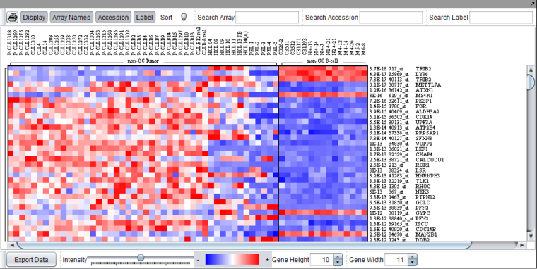
| − | The t-test result can also be displayed | + | The t-test result can also be displayed in the Color Mosaic component. |
(Visualization preference setting: Relative) | (Visualization preference setting: Relative) | ||
| − | [[Image: | + | [[Image:Color_Mosaic.png|{{ImageMaxWidth}}]] |
---- | ---- | ||
| Line 161: | Line 152: | ||
====Color Mosaic View==== | ====Color Mosaic View==== | ||
| − | (Visualization preference setting: | + | (Visualization preference setting: Relative) |
| − | |||
| − | |||
| + | [[Image:Color_Mosaic_ANOVA.png|{{ImageMaxWidth}}]] | ||
====Tabular View==== | ====Tabular View==== | ||
| − | [[Image: | + | [[Image:ANOVA_Tabular_View.png|{{ImageMaxWidth}}]] |
=== Hierarchical Clustering Dendrogram === | === Hierarchical Clustering Dendrogram === | ||
| Line 182: | Line 172: | ||
[[Image:T_SOM_result.png|{{ImageMaxWidth}}]] | [[Image:T_SOM_result.png|{{ImageMaxWidth}}]] | ||
| + | |||
| + | ---- | ||
| + | |||
| + | |||
| + | |||
| + | ===Consensus Clustering (GenePattern)=== | ||
| + | |||
| + | |||
| + | [[Image:Consensus_clustering_result_color_mosaic.png|{{ImageMaxWidth}}]] | ||
| + | |||
| + | |||
---- | ---- | ||
| Line 189: | Line 190: | ||
====K-Nearest Neighbors (KNN)==== | ====K-Nearest Neighbors (KNN)==== | ||
| − | [[Image: | + | [[Image:KNN_Parameters.png|{{ImageMaxWidth}}]] |
| − | |||
| − | |||
| − | |||
| − | |||
====Example of classifier result==== | ====Example of classifier result==== | ||
| Line 199: | Line 196: | ||
The classifiers return groups of markers to the Markers component: | The classifiers return groups of markers to the Markers component: | ||
| − | [[Image:Tutorial-GP_KNN-ClassPredictions.png | + | [[Image:Tutorial-GP_KNN-ClassPredictions.png]] |
---- | ---- | ||
| Line 224: | Line 221: | ||
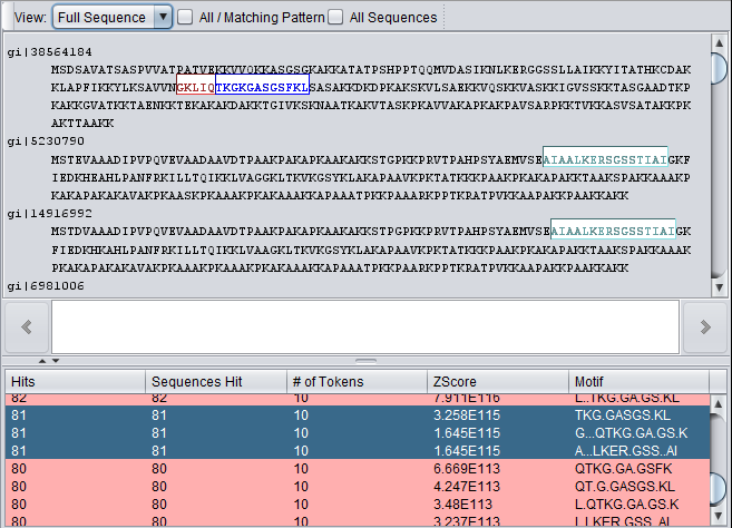
The Pattern Discovery component itself with results displayed in the sequence viewer. | The Pattern Discovery component itself with results displayed in the sequence viewer. | ||
| − | [[Image:PatternDiscovery_Basic_histone_result_exact_seqs.png | + | [[Image:PatternDiscovery_Basic_histone_result_exact_seqs.png]] |
====Position Histogram==== | ====Position Histogram==== | ||
| Line 230: | Line 227: | ||
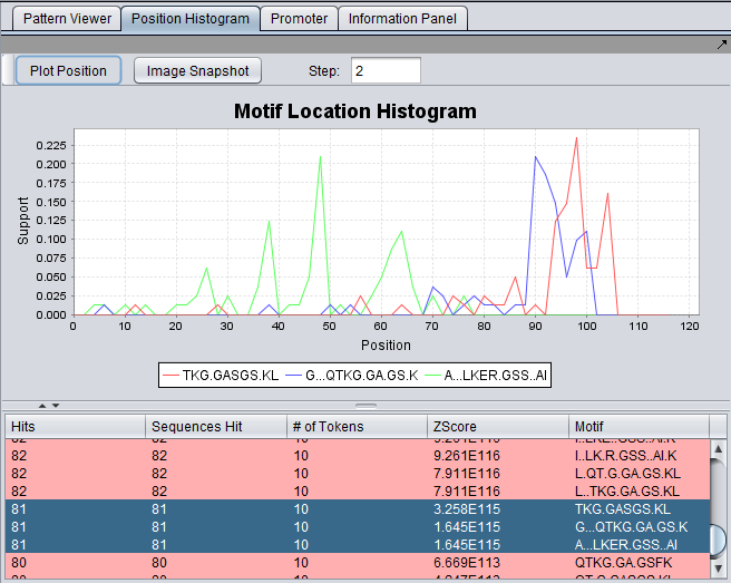
The Pattern Discovery component with results displayed as histogram of support for selected discovered motifs across the sequence data set. Support indicates what fraction of the seqeunces are matched by the motif at a within a sliding window about a given location. | The Pattern Discovery component with results displayed as histogram of support for selected discovered motifs across the sequence data set. Support indicates what fraction of the seqeunces are matched by the motif at a within a sliding window about a given location. | ||
| − | [[Image:PatternDiscovery_Basic_Histones_Result_exact_3_histogram.png | + | [[Image:PatternDiscovery_Basic_Histones_Result_exact_3_histogram.png]] |
---- | ---- | ||
| Line 247: | Line 244: | ||
====Sequence-level display of match==== | ====Sequence-level display of match==== | ||
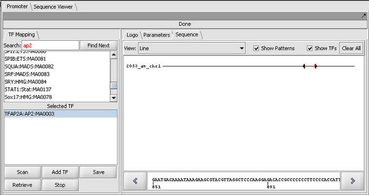
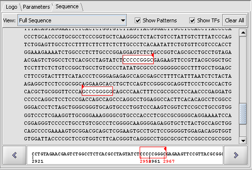
| − | [[Image:T_Promoter_CDH2_AP2_2000updn_scan_fullseq.png | + | [[Image:T_Promoter_CDH2_AP2_2000updn_scan_fullseq.png]] |
---- | ---- | ||
| Line 268: | Line 265: | ||
---- | ---- | ||
| − | ===Cellular Network Knowledge Base=== | + | ===Cellular Network Knowledge Base (CNKB)=== |
Results of queries against the CNKB can be filtered based on confidence values using the throttle graph. | Results of queries against the CNKB can be filtered based on confidence values using the throttle graph. | ||
| Line 285: | Line 282: | ||
===Master Regulator Analysis=== | ===Master Regulator Analysis=== | ||
| − | [[Image: | + | [[Image:MRA_viewer_GBM_FOSL2_v3.png|{{ImageMaxWidth}}]] |
| Line 314: | Line 311: | ||
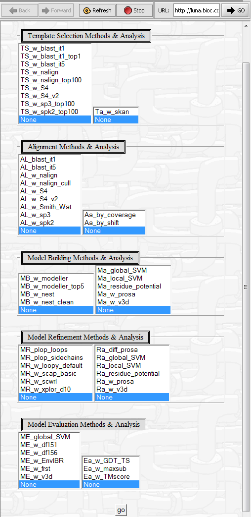
PUDGE allows a pipeline of modeling and evaluation steps, depicted below, to be set up and run. | PUDGE allows a pipeline of modeling and evaluation steps, depicted below, to be set up and run. | ||
| − | [[Image:T_Pudge_Parameters.png | + | [[Image:T_Pudge_Parameters.png]] |
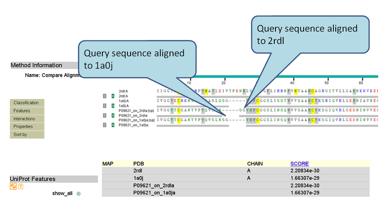
Pudge has a number of output types, the following illustrates a sequence alignment: | Pudge has a number of output types, the following illustrates a sequence alignment: | ||
Latest revision as of 16:01, 17 October 2013
Contents
- 1 Overview
- 2 geWorkbench Configuration
- 3 Workspace and Data Management
- 4 Microarray Data Displays
- 5 Gene and Pathway Annotations
- 6 Statistical tests, clustering and classification
- 7 Sequence Analysis / Pattern Discovery
- 8 Network Discovery and Visualization
- 9 Molecular Structure
Overview
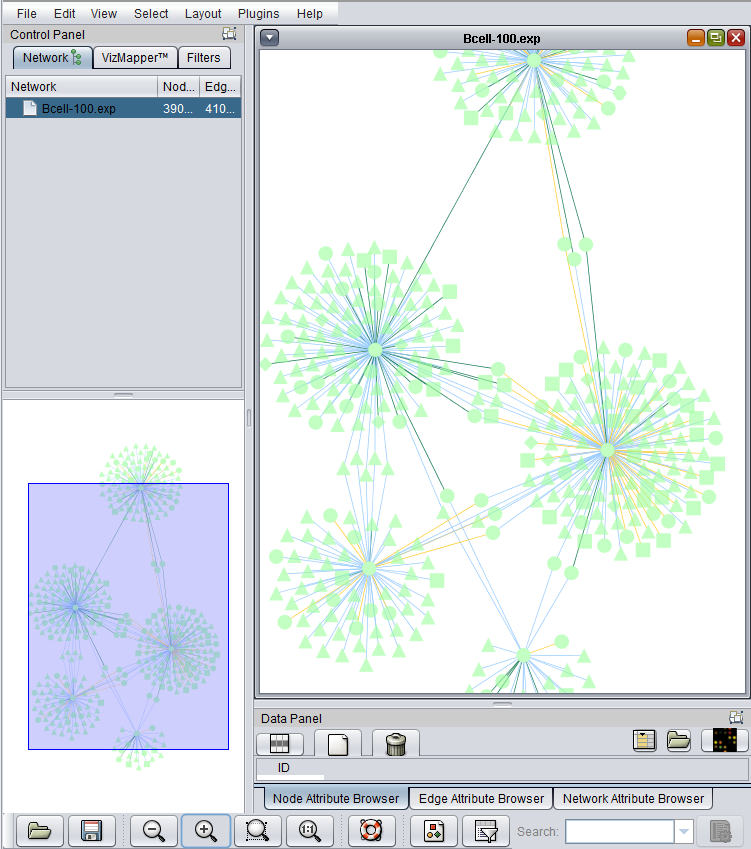
The geWorkbench graphical interface with a CNKB query result dislayed in Cytoscape.
geWorkbench Configuration
Component Configuration Manager
Individual components can be loaded as needed.
Workspace and Data Management
Workspace
Data sets are loaded into the Workspace. Individual analysis results are stored under their parent dataset.
Array/Phenotypes
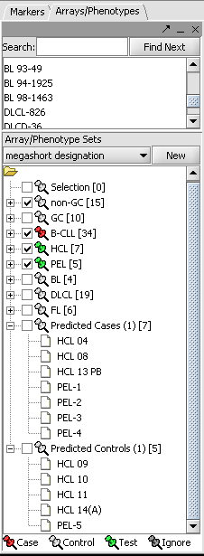
Sets of arrays can be defined and included or excluded from particular analyses (via checkboxes). Sets can be individually marked as belonging to case (here indicated with a red thumbtack) or control groups.
Markers
Sets of arrays can be defined and included or excluded from particular analyses (via checkboxes).
In addition, routines such as ANOVA or t-test return lists of significant markers to the Markers component.
Retrieval from caArray
Microarray data can be retrieved directly from instances of caArray.
Microarray Data Displays
Microarray Viewer
The Microarray Viewer displaying marker values for selected array.
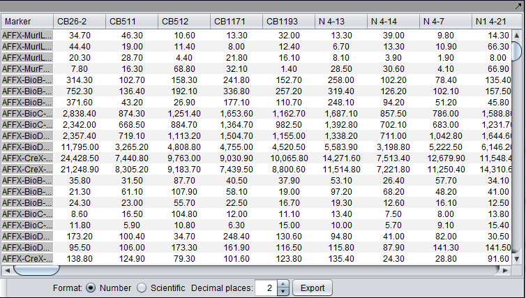
Tabular Microarray Viewer
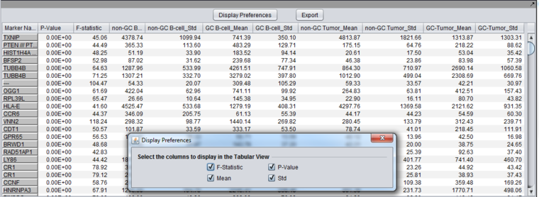
The Tabular Microarray Viewer displays expression values in spreadsheet format.
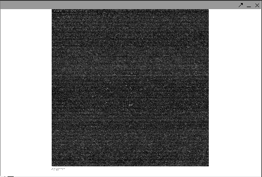
CEL Image Viewer
Allows viewing of Affyemtrix CEL files.
Color Mosaic
The Color Mosaic component displaying a result from ANOVA analysis. It can also directly display the loaded expression data, or subsets of that data created using Marker and Array sets.
Expression Profile
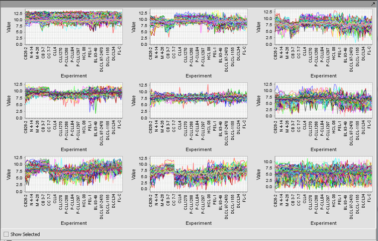
Expression Profile plotting values for selected markers and arrays. Individual values can be seen by hovering over a desired data point.
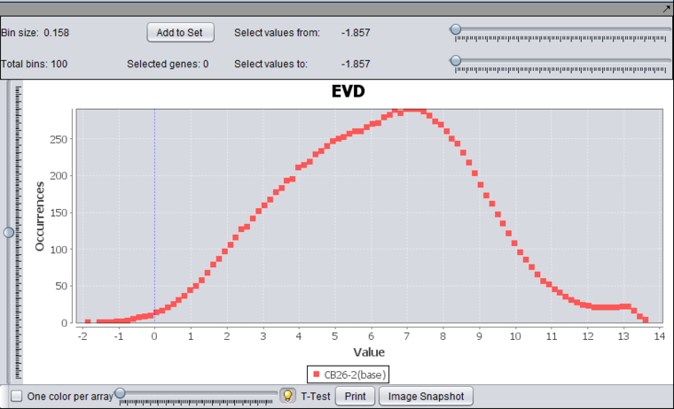
Expression Value Distribution
The dataset has been quantile normalized and log2 transformed.
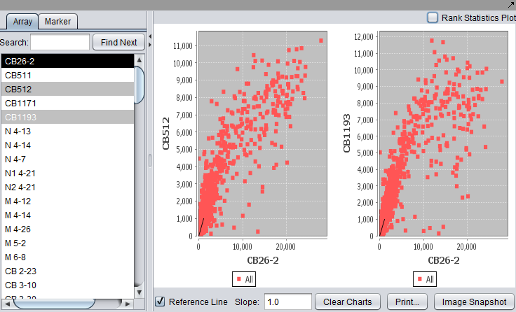
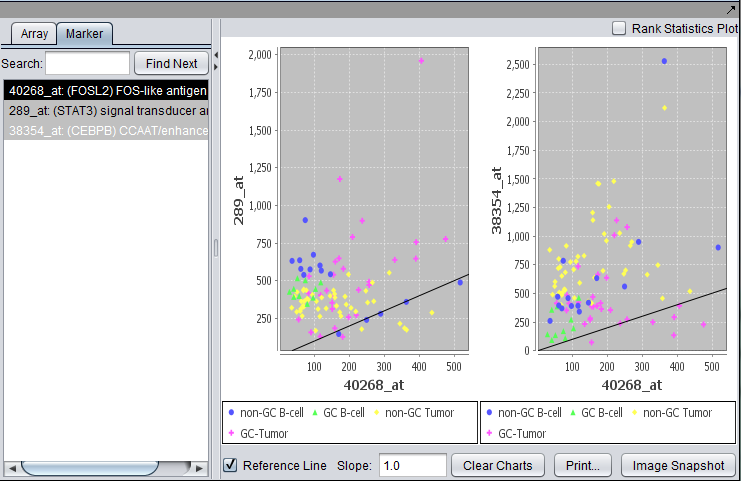
Scatter Plot
Compare multiple markers or arrays with the standard Scatter Plot analysis.
Array vs Array
Marker vs Marker
Gene and Pathway Annotations
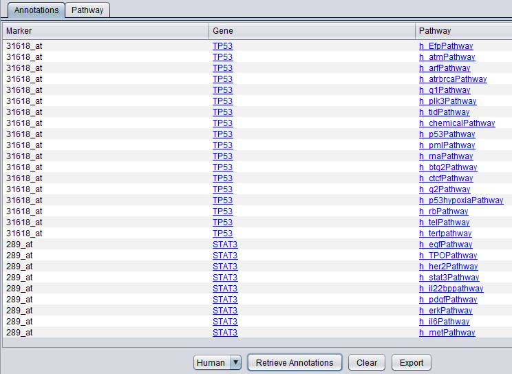
Marker Annotations
Retrieve and display gene and pathway information from bioDBNet.
Marker Annotations - BioCarta Pathways
Displays BioCarta images retrieved via bioDBNet.
Statistical tests, clustering and classification
Gene Ontology Term Over-representation Analysis
T Test
Volcano Plot
A t-test result display on a "volcano plot": Log significance vs log fold change.
Color Mosaic
The t-test result can also be displayed in the Color Mosaic component.
(Visualization preference setting: Relative)
Analysis of Variance (ANOVA)
Detects markers for which a statistically significant difference exists in a data set containing multiple classes of samples.
Color Mosaic View
(Visualization preference setting: Relative)
Tabular View
Hierarchical Clustering Dendrogram
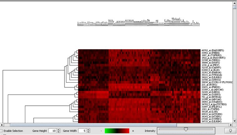
A Dendrogram displays the results of the Hierarchical clustering analysis.
SOM Clustering
Self Ordered Map clustering results are displayed as series of expression profiles corresponding to discovered groupings.
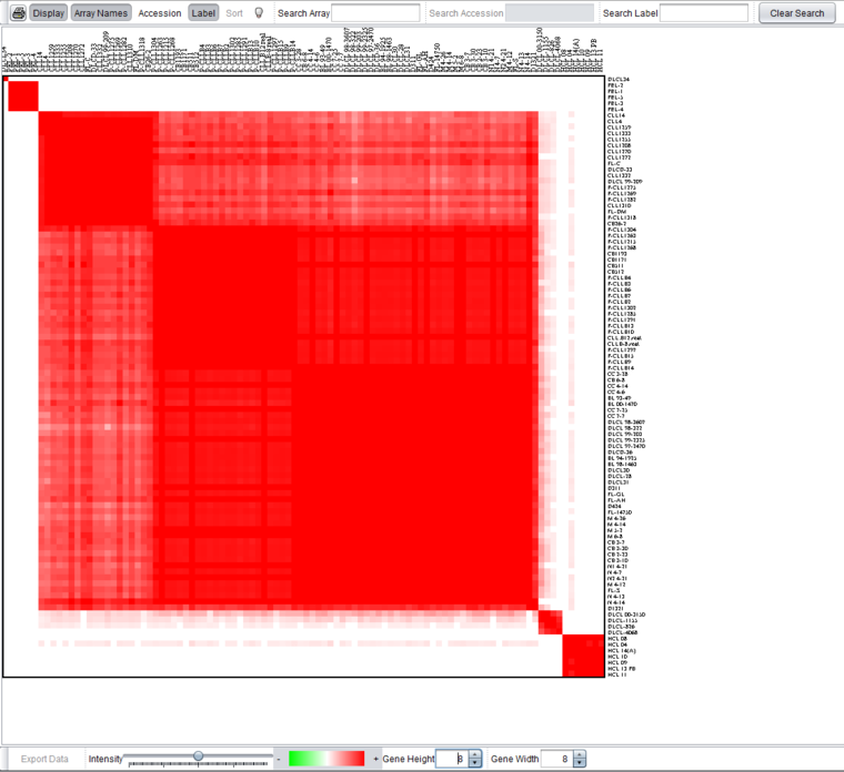
Consensus Clustering (GenePattern)
Classification (GenePattern)
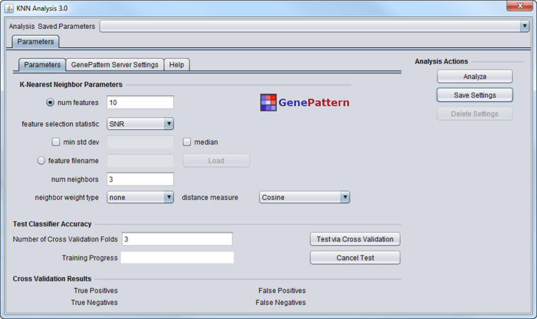
GenePattern components that perform classification on microarray datasets have been adapted to geWorkbench.
K-Nearest Neighbors (KNN)
Example of classifier result
The classifiers return groups of markers to the Markers component:
Sequence Analysis / Pattern Discovery
Sequence Retriever
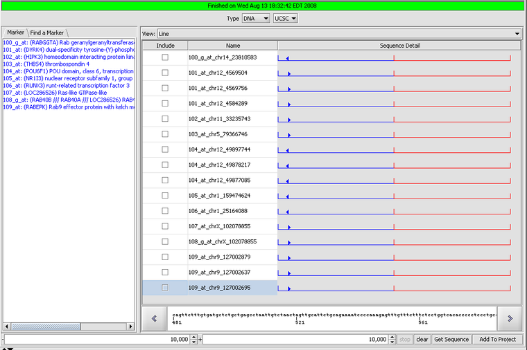
Retrieve genomic and protein sequences for selected markers. Retrieved sequences can be individually selected and added to the project as new data nodes.
BLAST Queries
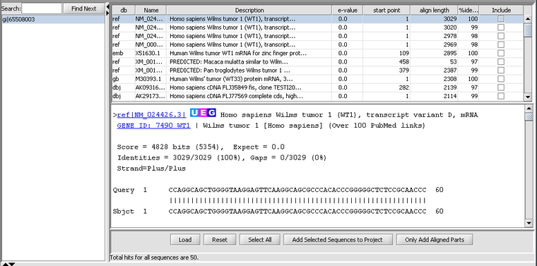
The Sequence Alignment component submits BLAST jobs to the NCBI server and displays the results such that individual hits can be used in further analysis steps.
Pattern Discovery
Use the SPLASH algorithm to discover sparse amino or nucleic acid patterns in a loaded sequence.
Motif discovery and display
The Pattern Discovery component itself with results displayed in the sequence viewer.
Position Histogram
The Pattern Discovery component with results displayed as histogram of support for selected discovered motifs across the sequence data set. Support indicates what fraction of the seqeunces are matched by the motif at a within a sliding window about a given location.
Promoter
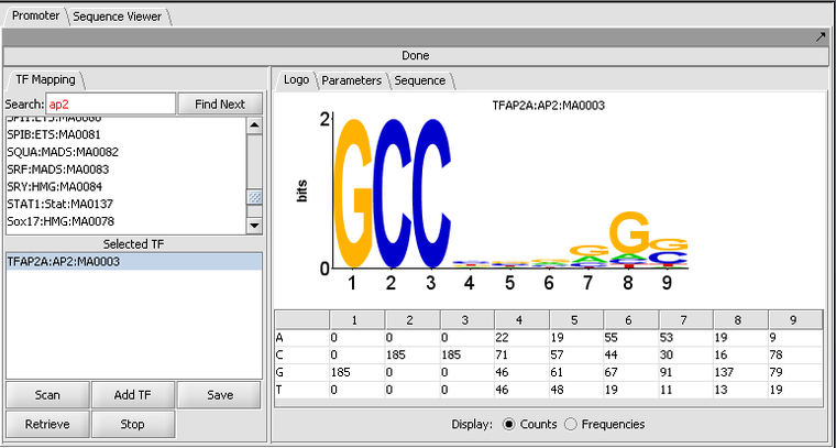
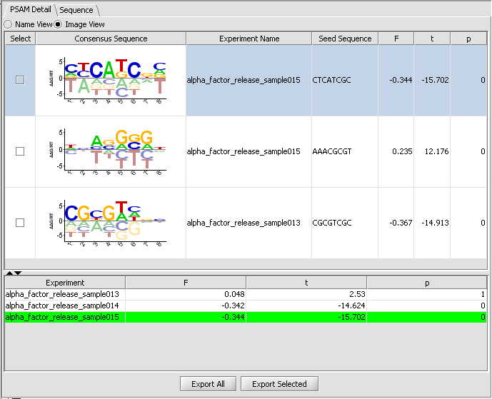
Individual motifs from the JASPAR Transcription Factor Binding Profile Database can be scanned against loaded genomic sequences.
Motif selection and Logo display
Result of a scan against a single sequence
Sequence-level display of match
MatrixREDUCE
MatrixREDUCE is a tool for inferring the binding specificity and nuclear concentration of transcription factors from microarray data.
Network Discovery and Visualization
Cytoscape - ARACNe Network display
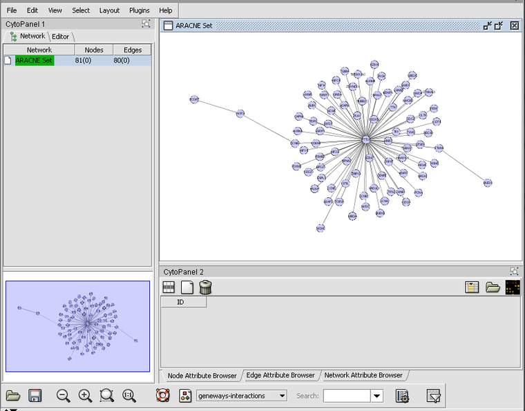
The adjacency matrix generated by an ARACNe network reverse engineering run displayed in Cytoscape.
Cellular Network Knowledge Base (CNKB)
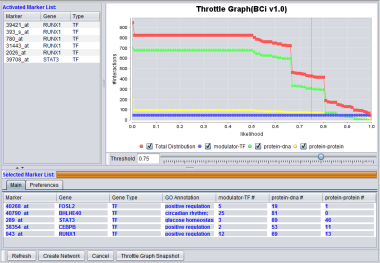
Results of queries against the CNKB can be filtered based on confidence values using the throttle graph.
Query results and Throttle Graph
CNKB query results displayed in Cytoscape
Display of CNKB interactions in Cytoscape.
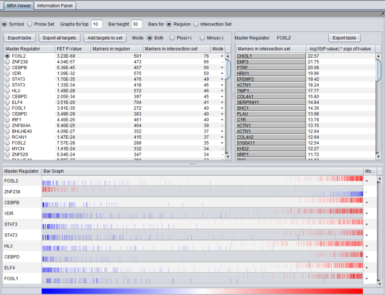
Master Regulator Analysis
Molecular Structure
JMOL Structure Viewer
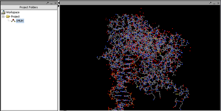
JMOL is a viewer for PDB protein structure files.
Mark-Us - Protein Functional Annotation
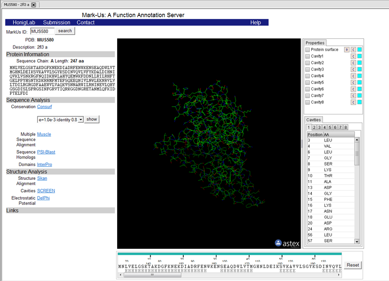
Mark-Us is a web server to assist the assessment of the biochemical function for a given protein structure. MarkUs identifies related protein structures and sequences, detects protein cavities, and calculates the surface electrostatic potentials and amino acid conservation profile.
PUDGE
Pudge is a server for the prediction of the 3D structures of proteins. While the server can be run without any user intervention, it is primarily designed to be interactive and to allow functional information to be used as a guide to the modeling.
PUDGE allows a pipeline of modeling and evaluation steps, depicted below, to be set up and run.
Pudge has a number of output types, the following illustrates a sequence alignment:
