Difference between revisions of "User:Smith"
| Line 106: | Line 106: | ||
| − | Hierarchical Clustering | + | ===Fast Hierarchical Clustering=== |
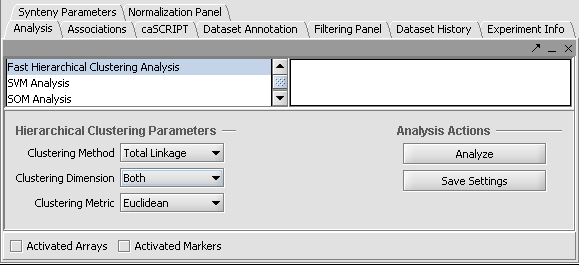
| + | '''Fast Hierarchical Clustering''' is found in the '''Analysis Panel'''. | ||
| + | |||
| + | In this example we shown Hierarchical Clustering being performed with the following options: | ||
| + | |||
| + | 1. Clustering Method: "Total Linkage" | ||
| + | |||
| + | 2. Clustering Dimension: "Both" | ||
| + | |||
| + | 3. Clustering Metric: "Euclidean" | ||
[[Image:T_Analysis_FHC.png]] | [[Image:T_Analysis_FHC.png]] | ||
| − | ''' | + | |
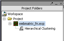
| + | Hit '''Analyze''' to run the clustering. The resulting dataset is inserted into the '''Project Panel''' | ||
| + | |||
| + | |||
| + | [[Image:T_ProjectFolder_HierarchClust.png]] | ||
| + | |||
| + | |||
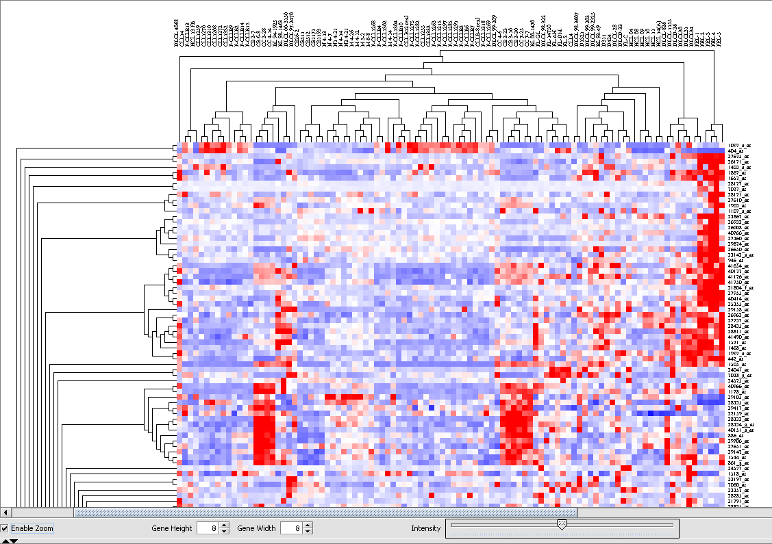
| + | and can be viewed in the '''Dendrogram Panel'''. | ||
| + | |||
[[Image:T_Dendrogram_Clusters.png]] | [[Image:T_Dendrogram_Clusters.png]] | ||
| − | |||
| − | [[Image:T_Dendrogram_SelectCluster | + | The cluster can be viewed by scrolling the window. Here we will pick an interesting cluster near the top for further investigation. |
| + | |||
| + | 1. Click '''Enable Zoom'''. | ||
| + | |||
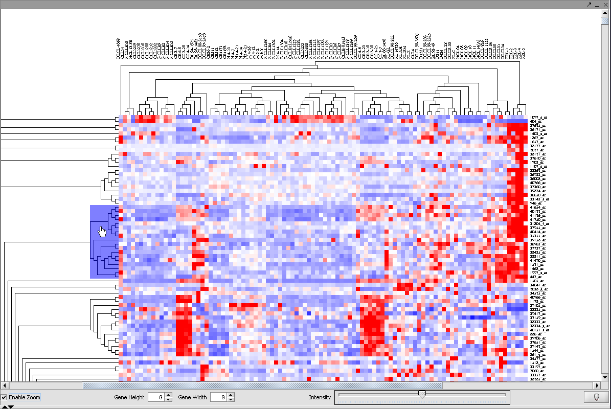
| + | 2. Position the mouse pointer over the cluster subtree of interest. It will be highlighted in blue. | ||
| + | |||
| + | |||
| + | [[Image:T_Dendrogram_SelectCluster.png]] | ||
| + | |||
| + | |||
| + | 1. Left click on the highlighted subtree to view it alone. | ||
| + | |||
| + | 2. By right clicking on the image, | ||
| − | |||
[[Image:T_Dendrogram_ClusterDetailAdd.png]] | [[Image:T_Dendrogram_ClusterDetailAdd.png]] | ||
| − | ''' | + | |
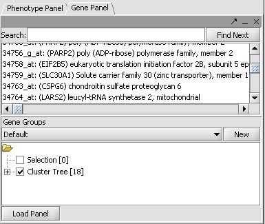
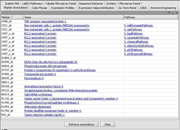
| + | this markers in this subtree can be added as a new marker panel to the '''Gene Panel.''' | ||
| + | |||
[[Image:T_GenePanel_ClusterTree.png]] | [[Image:T_GenePanel_ClusterTree.png]] | ||
| − | |||
| − | + | ||
'''separator''' | '''separator''' | ||
| − | [[Image:T_MarkerAnnotations_ClusterTree | + | [[Image:T_MarkerAnnotations_ClusterTree.png]] |
'''separator''' | '''separator''' | ||
Revision as of 17:55, 21 February 2006
Design and outline of tutorials for geWorkbench
Tutorial Design considerations - 1. Probably best not to use detailed section numbers, since we cannot autoupdate them in this wiki. Instead, rely on links? 2. Each section should list example data files needed, and these should be part of distribution.
Outline for tutorials
        2.1 Before You Begin
        2.2 Getting Started
             Is caWorkbench downloaded and installed?  Link to download and installation
             Important concepts:
                 Use of activated phenotype and marker panels throughout application.
                      - if no panels are activated, the "Activated Arrays" and "Activated Markers" check boxes should have no effect.
                      - if gene or phenotype panels are activated, then these check boxes should control what is used or displayed-
                       -- if one of the boxes is checked, only activated markers or arrays will be used.
                       -- if the box is not checked, then (in most cases - are there any exceptions?) the gene or phenotype panels will be ignored and all arrays or markers will be used.
                      Note that there is a new "plot" button that is available only when a gene panel is active.
             The  menu bar - point out that some commands are available both from the menu bar and by right-clicking on a dataset....
        2.3 Loading Data
             2.3.1 File types supported
                    Expression
                       Affymetrix MAS5/GCOS (text files output by Affymetrix software)
                       Affymetrix File Matrix (.exp)(a geWorkbench defined format)
                       RMAExpress Processed File
                       GenePix
                       Note - the type "Normalized no-confidence expression matix" has switched the phenotype and gene labels -don't use until fixed.
                    Genotypic
                       Genotypic data files - is this working?
                    Sequence
                       Fasta
                    Pattern Detection
                       Pattern Files
             2.3.2 Loading MAS5/GCOS type files
                        Use the 10 cardiomyopathy files from Harvard.
                        What happens the first time a new chip-type is loaded - how long does it take, what is happening, what internal files are being built?
             2.3.3 Merging loaded data

           [   These examples not really needed.....
             2.3.4 Loading matrix format files
                        Include webmatrix2000G?, webmatrix4000G? and webmatrix.exp?
                    Note - explain matrix format in an appendix
             2.3.5 Other file types supportedLoading RMAExpress files
                    Must generate an example RMAExpress file, start with harvard cardio files?
           ]
        2.4 Working with Marker and Phenotype Panels
                    Use the cardiomyopathy dataset created in 2.3
               2.4.1 Creating Phenotype Panels
               2.4.2 Assigning Case/Control status
               2.4.3 Activating a phenotype panel
               2.4.4 Creating Gene/Marker Panels
               2.4.5 Activating a phenotype panel
        2.5 Saving data files
               Use the cardiomyopathy dataset annotated in 2.4
               2.5.1 Save to matrix file
         2.6 Visualize Gene Expression
               Microarray Panel
                 Point out intensity and array sliders, color key and array name.
               Color Mosaic
                 Point out only displays when "Display" button pushed.
                 Point out intensity, accession, gene height and width controls.
                 ??Explain whether remaining controls work or not:  Pat,Abs,Ratio.???
               Expression Profiles
                 - displays expression level against array number. Each marker is a separate color line.
               Expression Value Distribution
                 - for a single array, plots expression value against marker number.
         2.6 Filter and Normalize Data
               2.6.1 Normalize
               2.6.2 Filter
         2.7 Clustering Gene Expression Data
         2.8 Differential Expression
               2.8.1 T Test
         2.9 Regulatory Network
         2.10 Integrated Annotation Information
         2.11 Enrichment Analysis
         2.12 Sequence Analysis
         2.13 Pattern Discovery
         2.14 Promoter Analysis
Tutorial: Hierarchical Clustering
Preliminary Filtering and Normalization
The file "webmatrix.exp" contains results from 100 Affymetrix HG-U95 chips containing B-cell samples from numerous different disease states (phenotypes). 12600 markers are represented. To prepare this dataset for clustering we will filter and normalize the data. The steps shown are just an example of how filtering and normalization can be used, and each dataset should be handled according to the type of analysis being undertaken and its goals.
For this dataset, we performed the following steps:
1. Applied Expression Threshold Filter to remove very low expression values in the range 0-20.
2. Applied the Missing Values Filter with a maximum number of missing values per marker of 2. (Deletes markers with more than 2 missing values). This reduced the number of markers to 6327.
3. Performed Quantile Normalization using Averaging Method of Mean Marker Profile.
4. Applied the Deviation Filter with Deviation Bound of 20 and Missing Values set to Marker Average.
5. Applied the Missing Values Filter as in (2), which further reduced the number of markers to 6270.
The resulting dataset was named webmatrix_fn.exp and is available for download.
Fast Hierarchical Clustering
Fast Hierarchical Clustering is found in the Analysis Panel.
In this example we shown Hierarchical Clustering being performed with the following options:
1. Clustering Method: "Total Linkage"
2. Clustering Dimension: "Both"
3. Clustering Metric: "Euclidean"
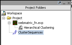
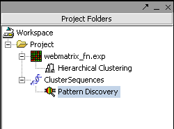
Hit Analyze to run the clustering. The resulting dataset is inserted into the Project Panel
and can be viewed in the Dendrogram Panel.
The cluster can be viewed by scrolling the window. Here we will pick an interesting cluster near the top for further investigation.
1. Click Enable Zoom.
2. Position the mouse pointer over the cluster subtree of interest. It will be highlighted in blue.
1. Left click on the highlighted subtree to view it alone.
2. By right clicking on the image,
this markers in this subtree can be added as a new marker panel to the Gene Panel.
separator
separator
separator
separator
separator
separator
separator
separator
separator
