Revision as of 17:50, 29 October 2009 (view source) Smith (talk | contribs) (→‎Working with and viewing the analysis results) ← Older edit		Revision as of 23:48, 29 October 2009 (view source) Smith (talk | contribs) Newer edit →
Line 1:		Line 1:
−	{{TutorialsTopNav}}	+	__NOTOC__
		+	__NOEDITSECTION__
	=Overview=		=Overview=

---

Revision as of 23:48, 29 October 2009

Overview

Regulatory activity in the context of specific cellular phenotypes can be modeled using interaction networks. These are graphs where nodes represent genes and an edge between two nodes A and B means that genes A and B are participants in the same regulatory activity. E.g., A can be a transcription factor for B; or, A can be an miRNA that silences B. Analysis of such regulatory networks [refs] has convincingly demonstrated their scale-free nature which is dominated by a relatively small number of nodes with a large degree of connectivity. The genes corresponding to those nodes are known as "master regulators" and collectively orchestrate the regulatory program of the underlying cellular phenotype(s).

The master regulator analysis (MRA) component in geWorkbench combines regulatory information from interaction networks with differential expression analysis. The objective is to place differentially expressed genes within a regulatory context and identify the master regulators responsible for coordinating their regulation, thus highlighting the regulatory apparatus driving phenotypic differentiation. Specifically, given an interaction network I, a (presumed) master regulator gene A, and two sets of microarrays representing two distinct phenotypes, MRA computes the intersection between two sets of genes:

1. The neighbors of A in the interaction network I (this gene set is called the regulon of A).
2. The set of differentially expressed genes in the array data from the two phenotypes of interest.

Fisher’s exact test is then used to quantify how likely it is to encounter an intersection of the observed size by chance alone. A small p-value is taken to imply that gene A may play a significant role in mediating the regulatory program that leads to the differential phenotypes.

Interaction networks are represented as "adjacency matrices". An adjacency matrix lists the connections that each node takes part in, and includes a measure of the strength of that interaction (e.g. the mutual information in the case of matrices generated by ARACNe).

Setting up an MRA run

Prerequisites

• First confirm that the MRA component is available in geWorkbench. If not, it can be loaded using the Component Configuration Manager.
• The MRA component will be listed along with the other analysis routines within the geWorkbench Analysis Panel.

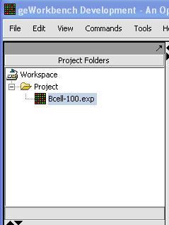
• Data from an expression experiment (comprising measurements from multiple arrays/samples) has been loaded and the corresponding node has been selected within the Project Folders:

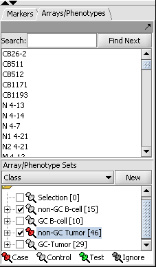
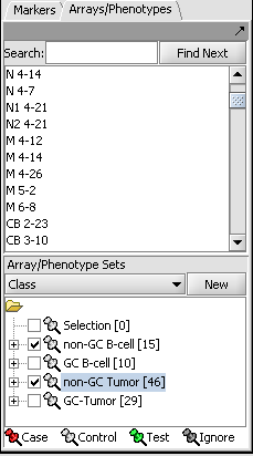
• Two array sets (each containing a distinct subset of arrays from the expression experiment) have been selected in the "Arrays/Phenotypes" component, representing the two phenotypes under investigation. One of the array sets (identified by the red-color pin) has been classified as containing the "Case" arrays (i.e., one of the 2 phenotypes) while the other one contains the "Controls" (the second phenotype):

NOTE:The "Case"/"Control" assignment is needed because, in general, it is possible to select more than one array sets for this analysis. In that case it is necessary to explicitly designate which belong to each of the 2 phenotypes.

Parameters and Settings

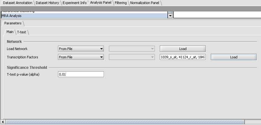
Load Network

There are 2 ways to designate the interaction network, represented by an adjacency matrix, that will be used for computing the regulons of the candidate master regulator genes:

• From File: by choosing a file that describes a network.
• From Project: by selecting an adjacency matrix node from the Project Folders component. Several analytical components in geWorkbench (e.g., ARACNE) produce adjacency matrix results nodes that can be utilized for this purpose.

Master Regulators

There are 2 ways to designate the candidate master regulator genes to use:

• From File: by choosing a file that contains a (comma separated) list of marker names.
• From Sets: by selecting a marker set from within the “Markers” component.

T-test p-value (alpha)

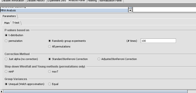
Differential expression between the 2 phenotypes of interest is assessed using a t-test. The p-value provided by the user indicates the significance threshold below which a gene’s average expression is presumed to be significantly different in the 2 sets of arrays (cases and controls). Additional parameter settings affecting the execution of the t-test are defined within the “T-test” subtab. The parameters specified there are exactly the same as those used for the differential expression t-test analysis (see description in the corresponding tutorial).

Working with and viewing the analysis results

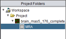
Following the successful completion of the MRA computation, a result node appears in the Project Folder area of the geWorkbench interface, under the microarray experiment node used for the computation:

The results of the analysis can be visualized in the MRA Viewer component by selecting the result node.

MRA Results Viewer

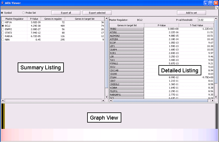
The MRA viewer is structured in 3 distinct areas.

Summary Listing

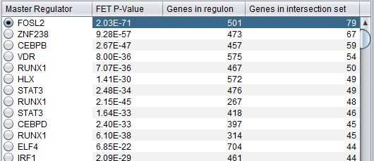
This is a table with one row for each candidate master regulator.

Each row contains 4 columns:

1. Master Regulator: This is either the master regulator gene name or the marker/probeset name identifying the corresponding array feature (depending on the selection of the radio buttons “Symbol” and “Probe set”).
2. P-value: the p-value from Fisher’s exact test. The test utilizes a 2x2 contingency table where rows classify markers as differentially expressed versus non-differentially expressed, while columns indicate if a marker belongs to the regulon of the master regulator or not. Counts are computed using all markers found in the input experiment data. (Fischer's exact test includes p-values for more-extreme tables).
3. Genes in regulon: The number of genes in the regulon of the master regulator (this comprises the set of genes that are first neighbors of the master regulator in the interaction network specified in the parameters panel).
4. Genes in target list: The number of differentially expressed genes that are also members of the regulon.

The contents of the table can be ordered by any column, by clicking on the column name.

Detailed Listing

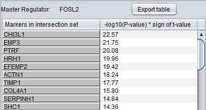
By clicking on the radio button associated with a master regulator in the Summary table, it is possible to display the complete listing of the differentially expressed genes intersecting the regulon of that master regulator.

The genes are displayed in a table with the following columns:

• Genes in target list: the names of the genes in the intersection set. Either the gene name or the marker/probe set name is used (based on the choice of "Symbol" or "Probe Set" radio buttons).
• P-value: the p-value of the t-test statistic for this marker, computed over the 2 sets of arrays (cases versus controls).
• T-test value: The actual value of the t-test statistic for the gene. A positive value indicates that the mean expression of the gene is higher in cases than in controls (a negative value has the opposite meaning).

The “P-val Threshold” parameter (located above the table) can be used to limit the number of target genes displayed. Specifically, only genes with a p-value less than the specified cutoff will be shown (if “P-val Threshold” is left empty, then all target genes in the intersection set are displayed). Additional functionality is made available through the following buttons:

• Add to Set: creates a set containing the markers that correspond to the genes currently displayed in the table. The new marker set appears in the Markers component and is named after the master regulator.
• Export selected: same as “Add to Set” but instead of being added to a marker set, the markers are stored into a file.
• Export all: stores into a file information for all master regulators (instead of only the one currently selected in the “Summary” view). Specifically, for each master regulator, the file lists the markers for all genes that are both differential expressed and also belong to the master regulator’s regulon.

Graph View

For a given master regulator A and the intersection between its regulon and the set of differentially expressed genes, the graph view helps assess if the intersection genes are preferentially over-expressed in the cases versus the controls. The biological motivation comes from observing [ref] that regulators with multiple targets tend to affect the expression level of (most of) their targets in one particular direction: they either promote their expression or inhibit it; but they rarely do both equally.

• The red-blue gradient at the bottom of the graph represents the range between the highest (red) and the lowest (blue) t-test statistic recorded among all differentially expressed genes.
• The vertical bars correspond to the genes displayed in the table under the “Detailed listing” portion of the interface, i.e., the intersection between the differentially expressed genes and the regulon of the master regulator A currently selected within the “Summary listing” table.
• The relative location of a bar on the gradient represents the t-test statistic recorded for the corresponding gene.
• Further, the color of each bar provides information about the correlation between the expression levels of the target gene and the master regulator A (correlations are computed as Pearson’s r, using data from all microarrays in the experiment): black means that the two genes are positively correlated (r > 0) while orange means that correlation is negative (r < 0).

Dataset History

Each results node stores the parameter settings used to setup the corresponding MRA run. The specific parameter values can be inspected within the Dataset History component, after clicking on the MRA results node in the Project Folders pane.

Example of running MRA

This example uses the Bcell-100.exp dataset available in the data/public_data directory of geWorkbench, and further described on the Download page. Briefly, this dataset is composed of 100 Affymetrix HG-U95Av2 arrays on which various B-cell lines, both normal and cancerous, were analyzed. Thus it explores a potentially wide variety of expression phenotypes.

Prerequisites

1. Obtain the annotation file for the HG-U95Av2 array type from the Affymetrix NetAffx website (http://www.affymetrix.com/support/technical/byproduct.affx?product=hgu95). The name will be similar to "HG_U95Av2.na29.annot.csv", where na29 is the version number. Loading the annotation file associates gene names and other information with the Affymetrix probeset IDs (see the geWorkbench FAQ for details on obtaining these files).
2. Store in your disk the following 2 files:
   1. Interaction_network.txt: describes an interaction network with 1955 nodes and 3810 edges. The file has 1955 lines (one for each node, the node name is the first entry in every line) and each line lists the edges emanating from that node. Edges are describes as tab-delimited pairs where the first member of the pair is the name of the target node and the second member is a number specifying a weight for the edge (MRA does not use the weight information but other geWorkbench components do). Node names correspond to marker ids.
   2. Master_regulators.csv: a list of master regulators. The marker ids in this file correspond to genes whose Gene Ontology annotation (under the Molecular Function category) lists them as transcription factors.

Loading and preparing the example data

1. Load the Bcell-100.exp dataset into geWorkbench as type "Affymetrix File Matrix". (See Local Data Files).
2. When prompted, load the annotation file.

Choosing array groups

The Bcell-100 dataset comes with predefined sets of arrays.

• In the Arrays/Phenotypes component (at lower left in the geWorkbench GUI), choose the group in the pulldown menu called "Class".
• Check the box beside the 2 array sets titled "non-GC B-Cell" and "non-GC Tumor", as shown in the figure below.

• Right-click on the array set titled "non-GC Tumor" and from the resulting popup menu choose "Classification->Case" to indicate that the arrays in that set will be treated as the "Case" phenotype for the t-test:

Setting up the parameters and starting MRA

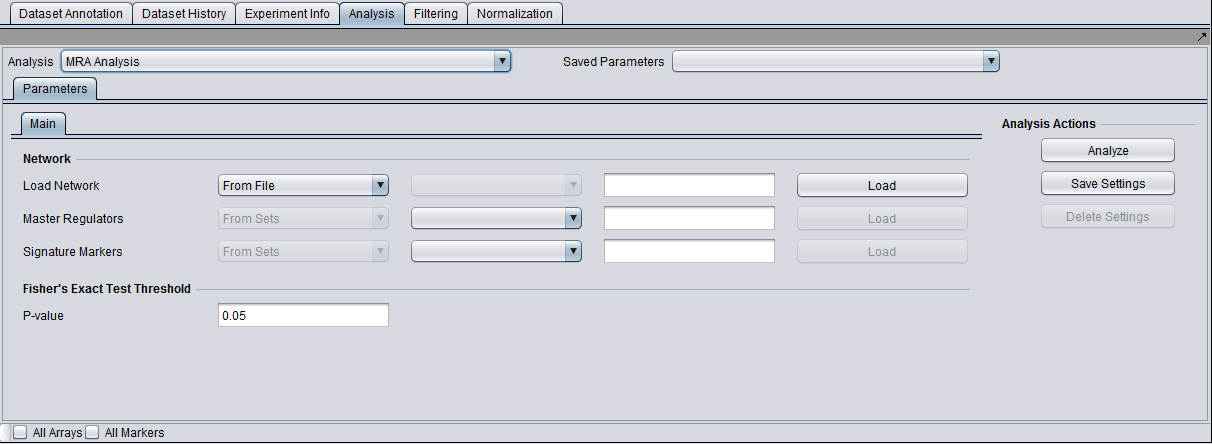
In the Analysis Panel, select the "MRA Analysis" entry and set the parameters as follows:

• Load Network: from the drop down choose the option "From File", click on the "Load" button, and select to open the file "Interaction_network.txt".
• Transcription Factors: from the drop down choose the option "From File", click on the "Load" button, and select to open the file "Master_regulators.csv".
• T-test p-value (alpha): set the significance threshold to 0.01.

• Click on the "T-test" tab and under Correction Method select the option titled "Standard Bonferroni", to indicate that the p-value of the t-test statistic for each gene should be family-wise corrected before compared to the p-value threshold (alpha) specified above.

• Click on the Analyze button.

Results

Upon completion of the analysis, an MRA results node is placed in the Project Folders tree. The analysis results can be browsed using the MRA viewer and are as shown above in the MRA Results Viewer section.

References