Difference between revisions of "User:Osborne"
m (→Analysis of Significant Genes) |
(→Analysis of Significant Genes) |
||
| Line 183: | Line 183: | ||
:In the previous steps we used a multiple-T-Test to determine which genes had significant differential gene expression. There are however other ways of doing this (such as ANOVA) which may be more appropriate. Additionally, a user may already have a list of genes of interest and be looking to conduct further analysis. This section describes the type of analysis that can be conduced on gene lists. | :In the previous steps we used a multiple-T-Test to determine which genes had significant differential gene expression. There are however other ways of doing this (such as ANOVA) which may be more appropriate. Additionally, a user may already have a list of genes of interest and be looking to conduct further analysis. This section describes the type of analysis that can be conduced on gene lists. | ||
| + | |||
| + | === Importing a Gene List === | ||
| + | In order to import a gene list, the first to be taken is to create a file that lists markers of interest - one marker for each line. For instance the following would be a legitimate file format: | ||
| + | 1552531_a_at | ||
| + | 1554726_at | ||
| + | 1560207_at | ||
| + | 1564684_at | ||
| + | |||
| + | |||
| + | It consists of 4 markers each on their own lines. To import this set of genes into geWorkbench do the following: | ||
| + | #Select the Markers panel in the middle left portion of the application | ||
| + | #Click on "Load Set" | ||
| + | #Select the file that contains the list of genes in the previously mentioned format. In our case it is a file called "ANOVAGeneList" and contains a set of genes identified as being differentially expressed from ANOVA analysis | ||
| + | #Press the Open Button | ||
| + | :This should result in a marker set being loaded and appearing in the "Marker Sets" in the bottom left portion of the screen as shown below. We can now use this marker set for subsequent analysis. | ||
=== Retrieving Annotations for Genes of Interest=== | === Retrieving Annotations for Genes of Interest=== | ||
| − | :Now that we have a list of significant genes for our T-Tests we want to be able to learn more about them. First we can locate the "gene list of our significant genes by selecting the Markers panel in the selection panel (not Arrays/Phenotypes). It will list the significant genes for each of the T-Tests. In this case we have 131, 161 and 178 genes for each of the 3 combinations as seen in the picture above. | + | :Now that we have a list of significant genes for our T-Tests (or loaded our own marker set from a different type of analysis) we want to be able to learn more about them. First we can locate the "gene list of our significant genes by selecting the Markers panel in the selection panel (not Arrays/Phenotypes). It will list the significant genes for each of the T-Tests. In this case we have 131, 161 and 178 genes for each of the 3 combinations as seen in the picture above. |
:To retrieve our list of annotations associated with these genes. | :To retrieve our list of annotations associated with these genes. | ||
# Click on the Marker Annotations Panel | # Click on the Marker Annotations Panel | ||
Revision as of 17:51, 31 August 2006
Contents
Microarray Analysis with geWorkbench
Getting Started
- Requirements (Windows/Mac/Linux OS, Java 1.5 installed, at least 512 MB RAM)
- Installation
Background
Correct and complete microarray analysis requires both an understanding of the actual experiment and the statistical and mathmatical tools being used. The tools and techniques being used will vary depending on the type of experiment and what knowledge the user hopes to gain from the experiment. Here we will describe a how to go about analyzing one of the most common types of microarray experiments - differential gene expression on Affymetrix arrays. Most of the techniques described should be suitable for other types of analysis when appropriately modified, but the user is cautioned against applying them blindly to their own data.
Introduction
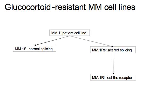
This tutorial walks the user through a fairly typical microarray experiment done using the Affymetrix HGU133Plus2 platform. In this case the experiments is a study of multiple myeloma resistance, it investigates 3 cell lines established from a patient resistant to glucocortoids. The 3 cell lines are:
- MM.1S expresses mostly the normal receptor. (C2E3)
- MM.Re expresses a small amount of normal receptor, but more alternatively spliced receptor (which is non-functional) (P1414)
- MM.1Rl expresses very little receptor of any kind. (P1310)
The goal is to get a baseline measurement to find the difference in expression between the three cell lines, no large difference is expected because they all orginate from the same ancestor. Splicing differences are expected.
Determining Genes with Significant Differential Expression
Data Inspection (optional)
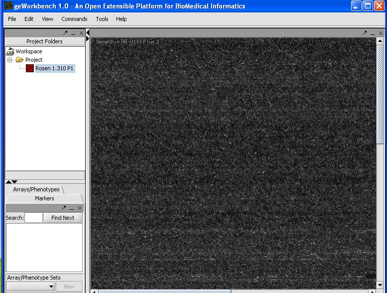
- The first step is to inspect visually a least one microarray. With the release of version 1.04 caWorkbench can now read in the Affymetrix CEL file format natively. However due to data structure incompatibility problems it can not yet do anything other than display the data unless it is pre-processed using R (geWorkbench can directly access an R server). The ability to see an image of the microarray is still useful, because it is worthwhile to make sure there are not obvious errors (streaking, etc...) on the microarray you are about to analyze. CEL files can be loaded by selecting type 'CEL' in the file loader. You should be able to see an image as shown below.
This image looks good, so we can continue. Inspect all of your images for defects if you want to be diligent. If you don't want to bother it is not usually a problem, but is may be worth doing if you run into problems later.
Data Preparation
- The next stepe is to prepare the data for loading. Affymetrix data is best imported into geWorkbench as tab-delimited files which contain 3 columns. The first column is the probeset identifier, the 2nd an optional annotation for the column, and the 3rd column contains the signal data. This file format is referred to in geWorkbench as "Affymetrix File Matrix" format and in order to be recognized by the file loading component of geWorkbench the filename should end with .exp. This is not to be confused with the Affymetrix .exp (experiment) file which is *not* loaded by geWorkbench. While this file cannot be directly generated from Affymetrix software, the CEL files or spreadhsheets that are generated by Affymetrix software can be modified into this format. Just use a spreadsheet program such as Excel.
- Generation from a spreadsheet
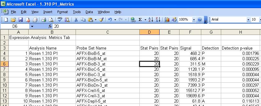
- The easiest way to get data from a small number of microarray files is to load in a file and modify in a spreadsheet program. Below is a result for a typical experiment.
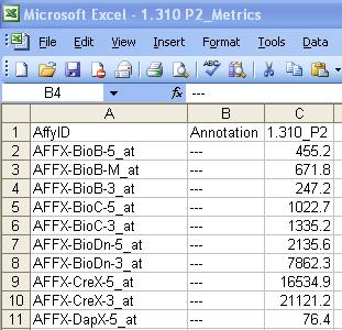
- The user should modify the spreadsheet to get it to look like the picture below. The 1st column title should be AffyID, the 2nd Annotation and the 3rd the name of the Microarray being analyzed.
- It should then be saved in tab delimited format with an .exp extension. This needs to be done for ALL microarrays in the experiment. If you are dealing with dozens or even hundreds of files, trying using R to generate the file instead.
- From CEL files
- FIXME (obsolete with 1.04)
Starting the Application
- On Windows click on Start -> Program -> geWorkbench 1.04
- We have no success running geWorkbench from the Mac or in Linux.
Load the data
- From the top part of the menu click on File -> New ->Project
- File -> Open
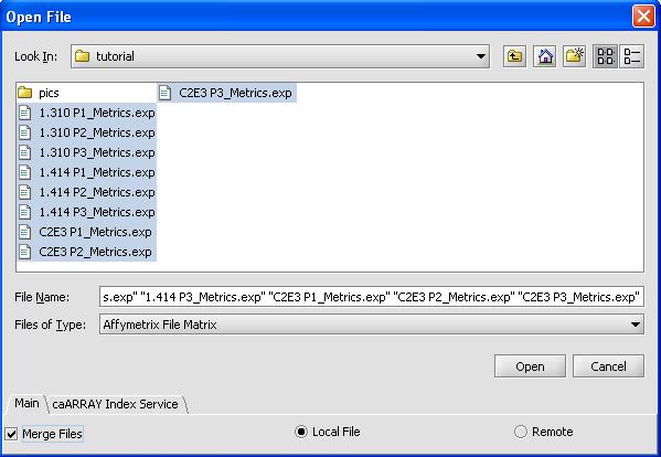
- Use the shift button to select all 9 files
- Click on the checkbox for merge files
- Select 'OK'. The loading dialog box is shown below.
- Select the appropriate chip type, most common Affy File types are provided. If your file type is missing you will have to add the
library files (downloaded from Affy's website) to the geWorkbench directory (FIXME - need more info)
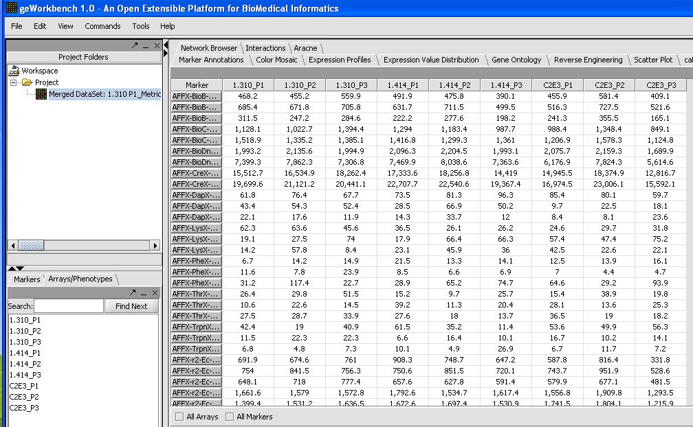
- With 9 chips from the HGU133Plus2 platform it will take a couple of minutes to load up. When you're done check and inspect that each of the chips was loaded successfully with the correct number. One quick way to do this is to look at the Microarray Tabular Viewer as shown below.
Log 2 Transform (optional)
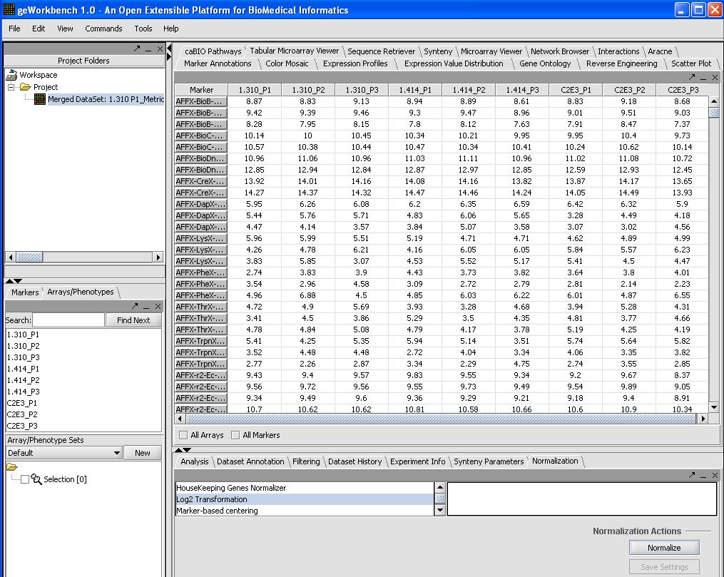
If your data has not been log2 transformed (our test data hasn't) it is a good idea to do so, the distribution is closer to normal on the log2 scale. To do this, follow the steps below.
- Select Normalizer from the bottom right hand portion of the screen
- Select Log2 Transformation
- Click on the normalization button
Normalize (optional)
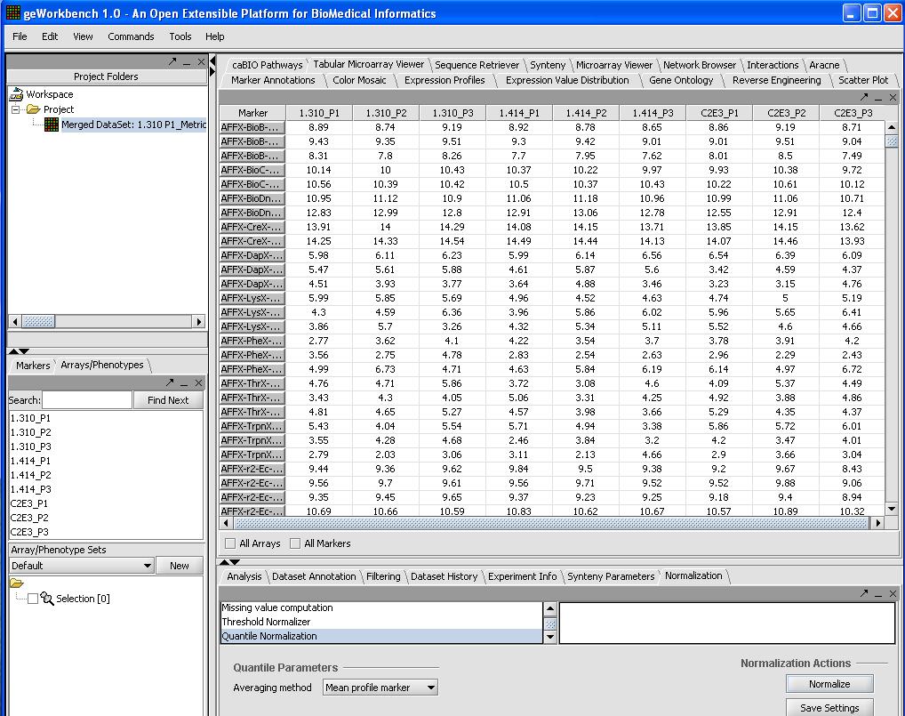
We will use quantile normalization to ensure the same expression value distribution across all the microarrays. In cases where the data has already been normalized by Affy's MAS5 algorithm this step is not required. If you desire quantile normalization it makes more sense to perform this on the raw (log2) transformed signal from the Affy.
To do so we will:
- Select Normalizer from the bottom right hand portion of the screen
- Select Quantile Normalization
- Select Mean Profiling to handle any missing values.
- Click on the Normalize button in the bottom right
A picture is shown below with the normalization window and the results of the normalization in the microarray tabular viewer.
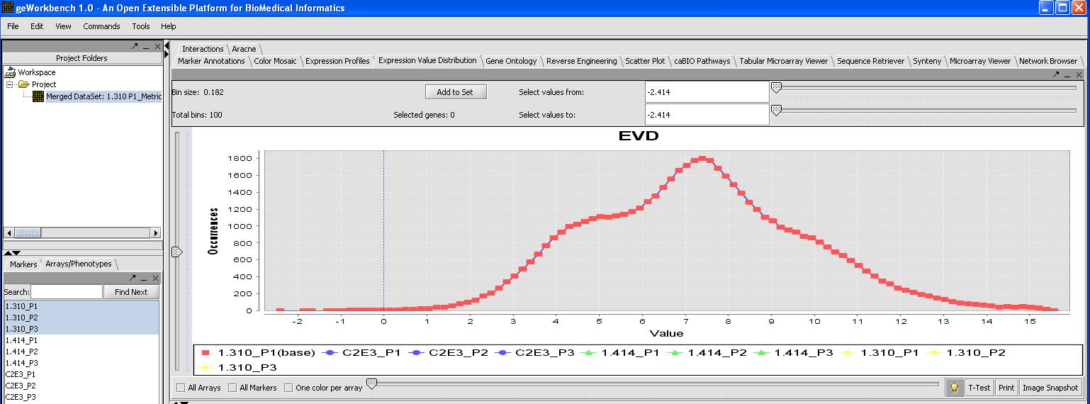
This can be verified by looking at the Expression Value Distribution plot, since quantile normalization should normalize expression across all microarrays. Click on the expression value distribution tab to verify that all the sets follow the same pattern.
Classification - Setting up controls and cases
In order for geWorkbench to garner some understanding of what the experiment is about, we need to set up our experimental classes. We have 3 different groups of data, wild type expression with C2E3, altered expression with P1.414 and low expression with P1.310. To classify our groups do the following:
- Use Shift and the left mouse button to select all 3 microarrays with P1.310 in the selection panel
- Right mouse click on this P1.310 set
- Select "Add to Set"
- Label this set as "Low" for low expression.
- Right mouse click on the "Low set" in the Arrays/Phenotypes window in the bottom left
- Select Classification -> Case to assign this set as a test case.
- Repeat the previous steps with the 3 microarrays for P1.414, setting them as a case as well. Label this set "Altered".
- Repeat the first 4 steps with the 3 C2E3 and label the set as "Wildtype". It does not need to be set as a control, this is the default option.
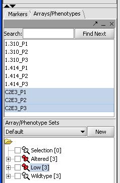
At the end the classification the Arrays/Phenotypes box should like the image below:
T-Test - Finding differentially expressed genes
Now that we have our samples classified we are going to do a simple T-Test to locate genes that are differentially expressed. A T-Test only compares 2 cases so we will first start by looking at differences between the Wildtype Control (C2E3) and the Altered (P1.414) Gene Expression Set.
- Click on the Analysis tab in the bottom right window and select T-Test. There should be 3 separate tabs for a T-Test - Degree of Freedom, P-Value Parameters and Alpha Correction as shown below.
- In the Degree of Freedom tab leave the default Welch Approximation for variances.
- In the P-Value Parameters tab change the default from 0.01 to 0.05. With our correction method we will not get any results with such a P-Value.
- In the Alpha Correction tab change select the correction method.
- Selecting none will give many results
- Selecting the severe Bonferroni or adjusted Bonferroni correction method will give no results.
- Activate the Wildtype and Altered expression set by clicking in the check box to the left of the set name in the bottom left set panel.
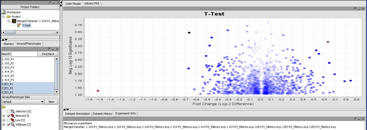
- Select the Analyze button (results should finish in a few seconds). The resulting T-Test result should appear in the project window below the data set and look like the results below.
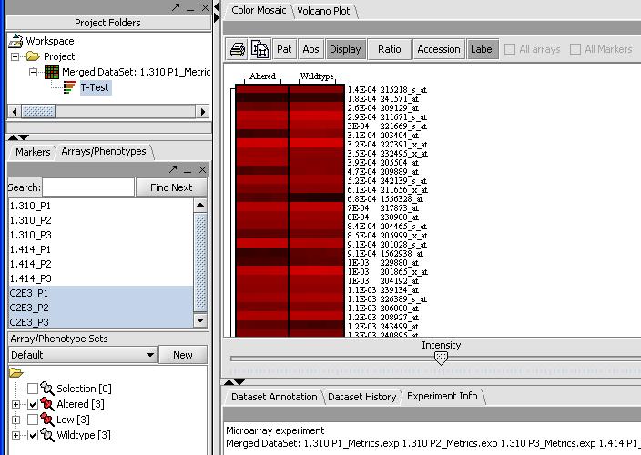
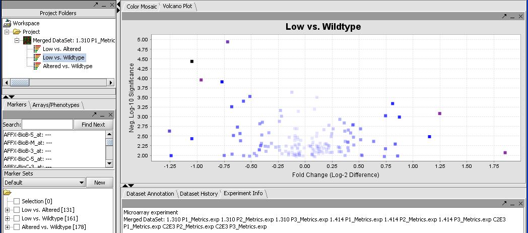
By mousing over the dots you can identify the individual probes responsible for that value. To get a more comprehensive list, investigate the color mosaic by selecting the Color Mosaic tabbed pane in the upper middle portion of the main panel. Results are shown below.
FIXME - I get 0 significant genes with this method, but I get 273 with no correction. I thought everybody uses some form of correction these days, I know Bonferroni is strict but....
(Show a page with the significant genes in the box)
Multiple T-Tests
Ideally because we have 3 separate classes of data we would like to do an ANOVA test to find our significant genes. geWorkbench does not support ANOVA but it does allow for multiple easy T-Testing. To do this:
- In the "Analysis" tab in the bottom right panel select Multi-T-Test from the list.
- Select the the critical value to be 0.01
- Select all 3 sets (the wildtype expression of C2E3, the altered expression of 1.414, and the low expression of 1.313) in the "Compare Panels" tab of the Multi-T-Test. Prior to running the T-Tests the panel should look like the one below.
- Now Select Analyze to run the tests
- 3 Seperate T-Tests should be run
- T-Test results for all 3 appear in the project window
Analysis of Significant Genes
- In the previous steps we used a multiple-T-Test to determine which genes had significant differential gene expression. There are however other ways of doing this (such as ANOVA) which may be more appropriate. Additionally, a user may already have a list of genes of interest and be looking to conduct further analysis. This section describes the type of analysis that can be conduced on gene lists.
Importing a Gene List
In order to import a gene list, the first to be taken is to create a file that lists markers of interest - one marker for each line. For instance the following would be a legitimate file format: 1552531_a_at 1554726_at 1560207_at 1564684_at
It consists of 4 markers each on their own lines. To import this set of genes into geWorkbench do the following:
- Select the Markers panel in the middle left portion of the application
- Click on "Load Set"
- Select the file that contains the list of genes in the previously mentioned format. In our case it is a file called "ANOVAGeneList" and contains a set of genes identified as being differentially expressed from ANOVA analysis
- Press the Open Button
- This should result in a marker set being loaded and appearing in the "Marker Sets" in the bottom left portion of the screen as shown below. We can now use this marker set for subsequent analysis.
Retrieving Annotations for Genes of Interest
- Now that we have a list of significant genes for our T-Tests (or loaded our own marker set from a different type of analysis) we want to be able to learn more about them. First we can locate the "gene list of our significant genes by selecting the Markers panel in the selection panel (not Arrays/Phenotypes). It will list the significant genes for each of the T-Tests. In this case we have 131, 161 and 178 genes for each of the 3 combinations as seen in the picture above.
- To retrieve our list of annotations associated with these genes.
- Click on the Marker Annotations Panel
- Activate our significant gene list by selecting Low versus Altered from the Marker Set panel in the bottom left. Activate by left mouse clicking on the checkbox.
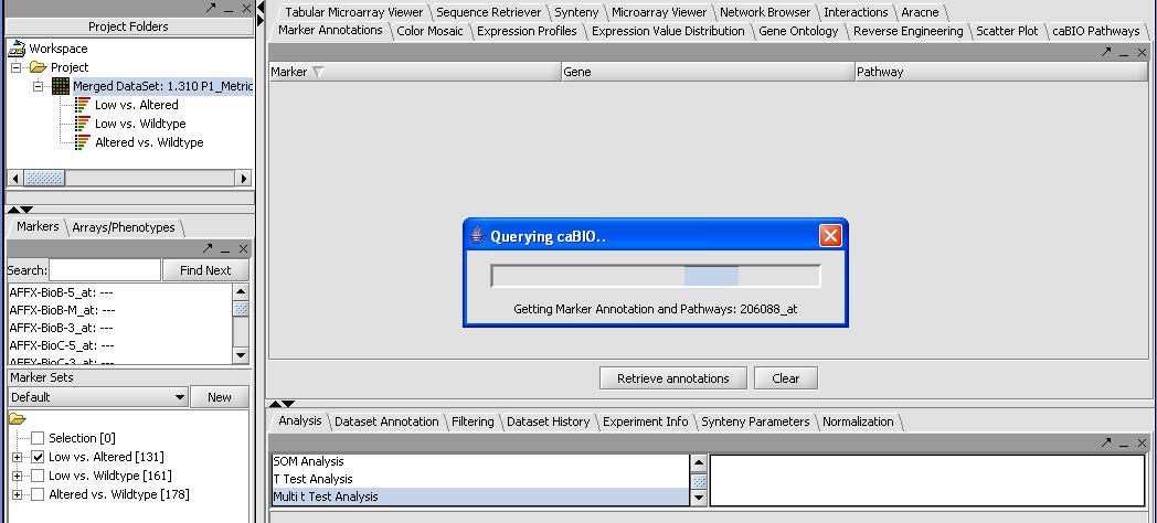
- Press the Retrieve Annotations button on the Annotations Panel. This steps requires a functional internet connection since annotations are retrieved from caBIO. If it is working you should get a screen similar to the one below. It can take a few minutes to retrieve the annotations for all 131 genes.
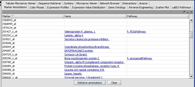
Once it has completed, the results will be automatically displayed in tabular format as shown below.
- Not all genes will have results, and even fewer genes will have pathway results. Clicking on the column titles will allow sorting of the pathways. Clicking on an individual gene result will open a web page describing the gene. Doing the same for a pathway result will not open a webpage, but will populate the caBIO Pathways panel. As an example:
- Left mouse click on the Pathways Column title to bring all pathway results to the top of the list
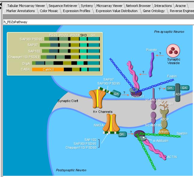
- Left mouse click on the h_PDZs_Pathway
- Select the caBIO Pathway tab. You should see the SVG image below in the panel.
Gene Ontology (GO) Analysis
The Gene Ontology can be used to discover annotation similarities between significant genes.
- Currently this functionality is no longer working with geWorkbench 1.04....
Promoter Analysis
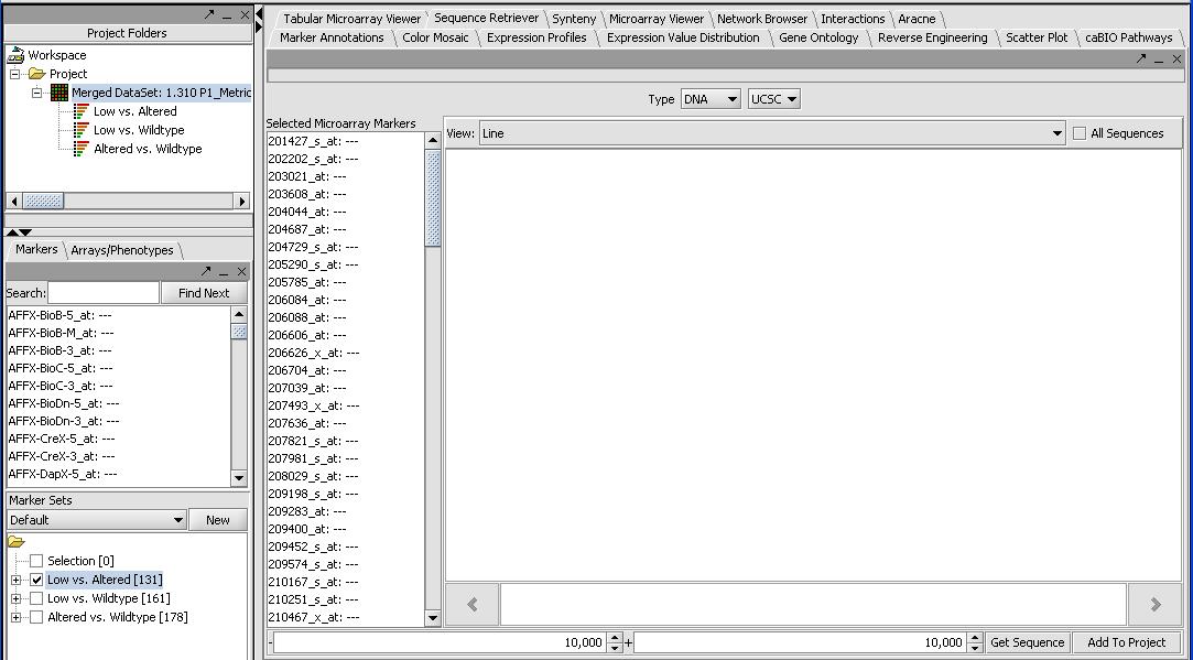
In order to look for common or potentially significant promoters in our list of significant genes a wide variety of promoter motifs are available for searching with. To do a basic promoter analysis do the following.
- Retrieve Sequences
- Click on the Sequence Retrieiver Panel
- Select the genes of sequence to retreive, make sure DNA is set as the return type
- Click "Get Sequences"
- Select the desired genomic build (for instance hg18 for the human genome) from the drop down menu
- Wait for the sequences to be retrieved
- Currently this functionality is no longer working with geWorkbench 1.04....
- Select promoter models
- etc...
