geWorkbench

Basic Microarray Analysis with geWorkbench

Getting Started

1. Requirements (Windows/Mac/Linux OS, Java 1.5 installed, at least 512 MB RAM)
2. Installation
   1. geWorkbench downloads
   2. Java downloads

Background

Correct and complete microarray analysis requires both an understanding of the actual experiment and the statistical and mathmatical tools being used. The tools and techniques being used will vary depending on the type of experiment and what knowledge the user hopes to gain from the experiment. Here we will describe a how to go about analyzing one of the most common types of microarray experiments - differential gene expression on Affymetrix arrays. Most of the techniques described should be suitable for other types of analysis when appropriately modified, but the user is cautioned against applying them blindly to their own data.

Introduction

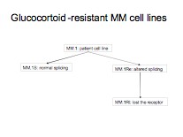
This tutorial walks the user through a fairly typical microarray experiment done using the Affymetrix HGU133Plus2 platform. In this case the experiments is a study of multiple myeloma resistance, it investigates 3 cell lines established from a patient resistant to glucocortoids. The 3 cell lines are:

1. MM.1S expresses mostly the normal receptor. (C2E3)
2. MM.Re expresses a small amount of normal receptor, but more alternatively spliced receptor (which is non-functional) (P1414)
3. MM.1Rl expresses very little receptor of any kind. (P1310)

The goal is to get a baseline measurement to find the difference in expression between the three cell lines, no large difference is expected because they all orginate from the same ancestor. Splicing differences are expected.

Step 1 - Inspect your data

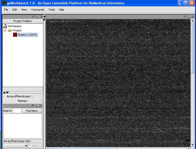
The first step is to inspect visually a least one microarray. With the release of version 1.04 caWorkbench can now read in the Affymetrix CEL file format natively. However due to data structure incompatibility problems it can not yet do anything other than display the data unless it is pre-processed using R (geWorkbench can directly access an R server). The ability to see an image of the microarray is still useful, because it is worthwhile to make sure there are not obvious errors (streaking, etc...) on the microarray you are about to analyze. CEL files can be loaded by selecting type 'CEL' in the file loader. You should be able to see an image as shown below.

This image looks good, so we can continue. Inspect all of your images for defects if you want to be diligent. If you don't want to bother it is not usually a problem, but is may be worth doing if you run into problems later.

Step 2 Data Preparation

The next stepe is to prepare the data for loading. Affymetrix data is best imported into geWorkbench as tab-delimited files which contain 3 columns. The first column is the probeset identifier, the 2nd an optional annotation for the column, and the 3rd column contains the signal data. This file format is referred to in geWorkbench as "Affymetrix File Matrix" format and in order to be recognized by the file loading component of geWorkbench the filename should end with .exp. This is not to be confused with the Affymetrix .exp (experiment) file which is *not* loaded by geWorkbench. While this file cannot be directly generated from Affymetrix software, the CEL files or spreadhsheets that are generated by Affymetrix software can be modified into this format. Just use a spreadsheet program such as Excel.

1. Generation from a spreadsheet

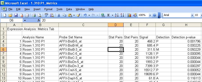
The easiest way to get data from a small number of microarray files is to load in a file and modify in a spreadsheet program. Below is a result for a typical experiment.

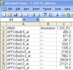
The user should modify the spreadsheet to get it to look like the picture below. The 1st column title should be AffyID, the 2nd Annotation and the 3rd the name of the Microarray being analyzed.

It should then be saved in tab delimited format with an .exp extension. This needs to be done for ALL microarrays in the experiment. If you are dealing with dozens or even hundreds of files, trying using R to generate the file instead.

1. From CEL files

FIXME (obsolete with 1.04)

Starting the Application

On Windows click on Start -> Program -> geWorkbench 1.04

We have no success running geWorkbench from the Mac or in Linux.

Load the data

1. From the top part of the menu click on File -> New ->Project
2. File -> Open
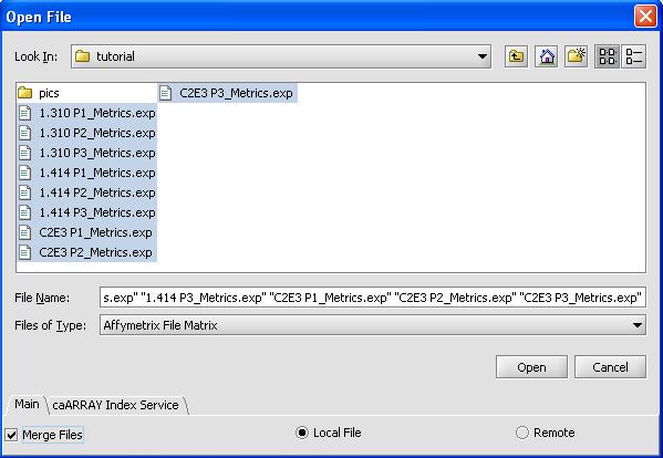
   1. Use the shift button to select all 9 files
   2. Click on the checkbox for merge files
   3. Select 'OK'. The loading dialog box is shown below.

1. 1. Select the appropriate chip type, most common Affy File types are provided. If your file type is missing you will have to add the

library files (downloaded from Affy's website) to the geWorkbench directory (FIXME - need more info)

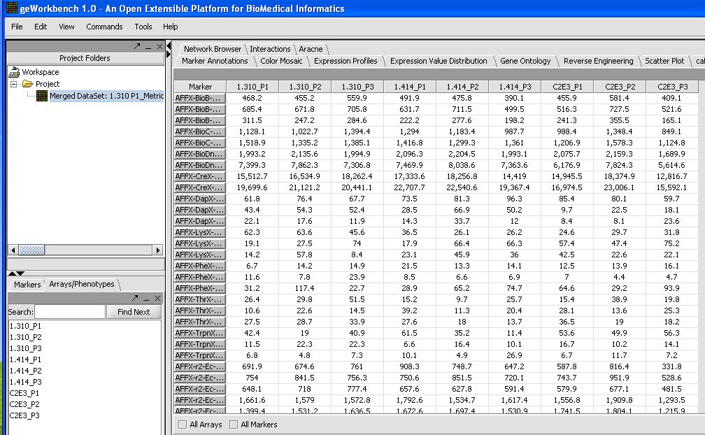
1. 1. With 9 chips from the HGU133Plus2 platform it will take a couple of minutes to load up. When you're done check and inspect that each of the chips was loaded successfully with the correct number. One quick way to do this is to look at the Microarray Tabular Viewer as shown below.

Log 2 Transform (optional)

1. Select Normalizer from the bottom right hand portion of the screen
2. Select Log2 Transformation
3. Click on the normalization button

Normalize

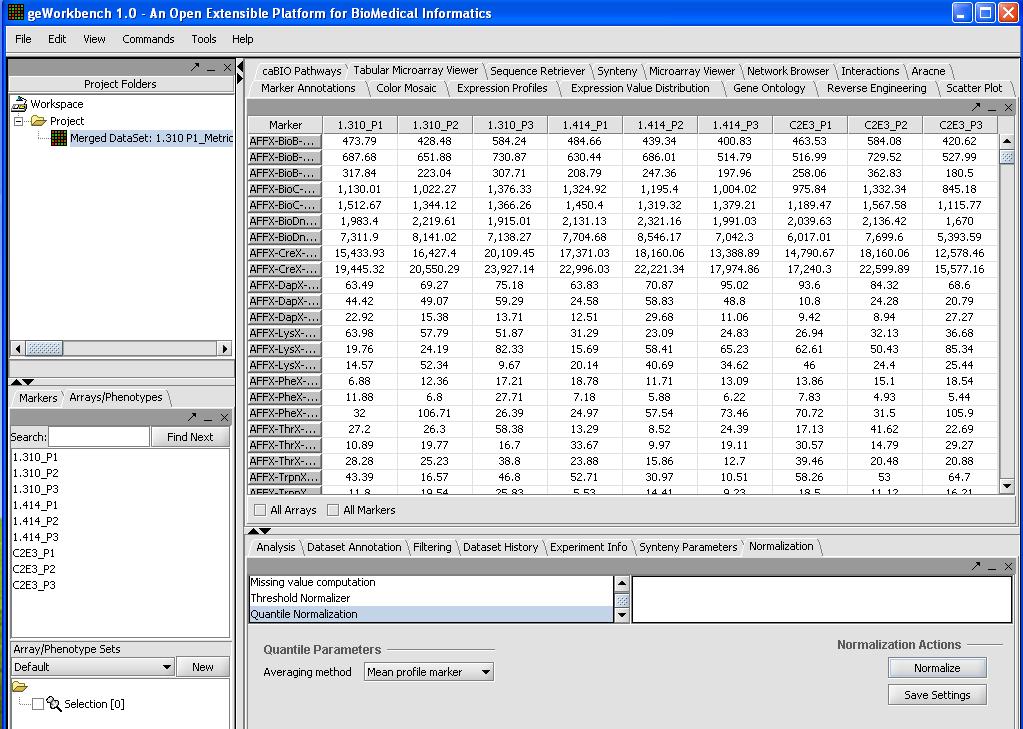
We will use quantile normalization to ensure the same expression value distribution across all the microarrays. To do so we will:

1. Select Normalizer from the bottom right hand portion of the screen
2. Select Quantile Normalization
3. Select Mean Profiling to handle any missing values.
4. Click on the Normalize button in the bottom right

A picture is shown below with the normalization window and the results of the normalization in the microarray tabular viewer.

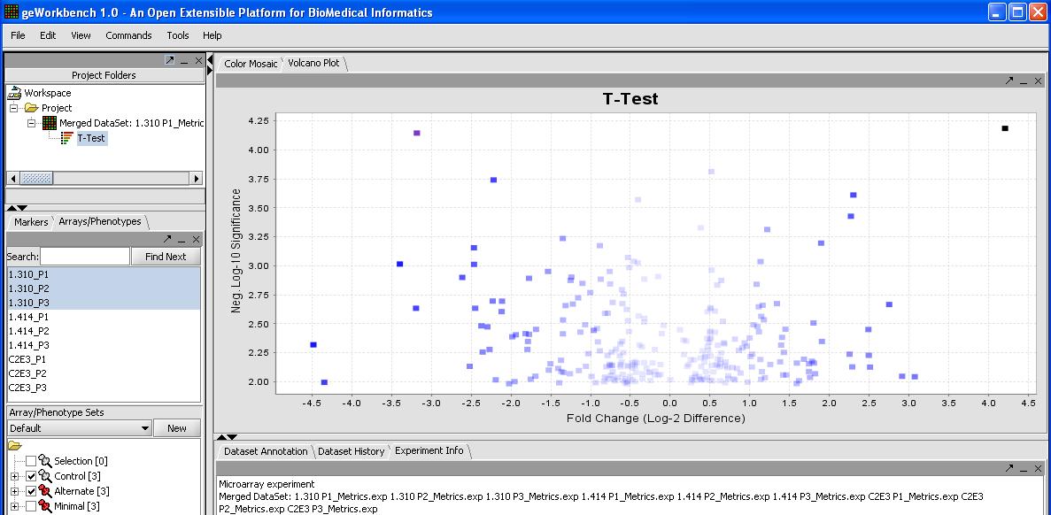
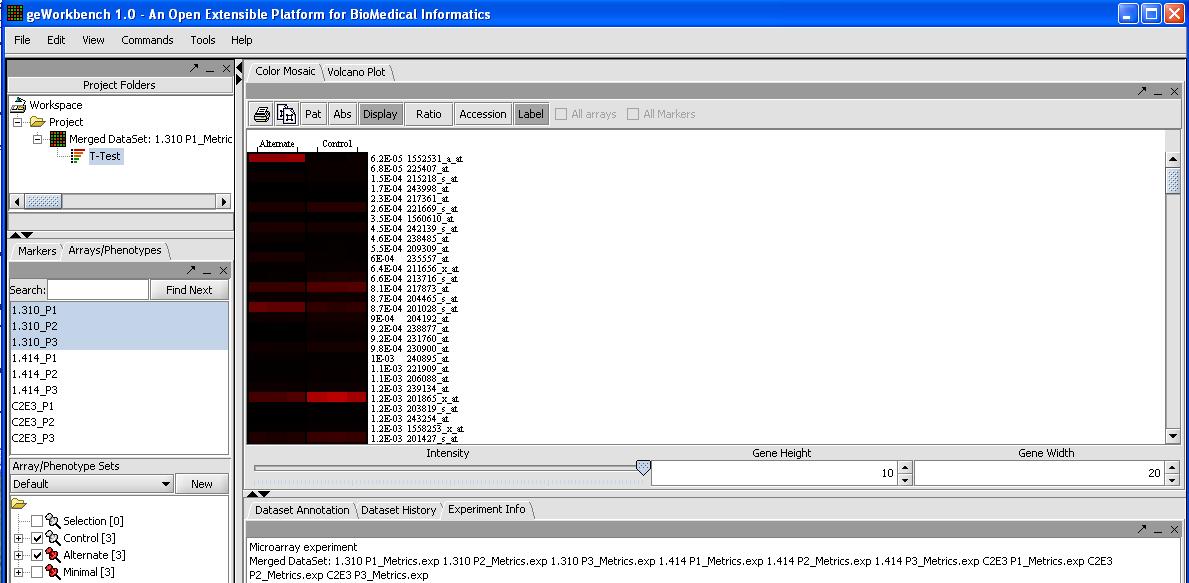
T-Test

1. Use Shift and the left mouse button to select all 3 microarrays with P1.310 in the selection panel
2. Right mouse click on this P1.310 set
3. Select Classification -> Case to assign this set as a test case
4. Repeat with the set of 3 microarrays for P1.414, setting them as a case as well
5. Select T-Test
6. Select correction method

Pattern Discovery

1. Other Analysis