Difference between revisions of "GeWorkbench-web/T-Test"
(Created page with "{{TutorialsTopNav}} =Overview= A t-Test analysis can be used to identify markers with statistically significant differential expression between two sets of microarrays. In ge...") |
m (moved T-Test web to GeWorkbench-web/T-Test) |
||
| (10 intermediate revisions by the same user not shown) | |||
| Line 1: | Line 1: | ||
| − | {{ | + | {{Template:GeWorkbench-webTutorialsTopNav}} |
| Line 11: | Line 11: | ||
| − | After the t-test is run, the markers meeting the | + | After the t-test is run, the markers meeting the significance threshold will be displayed graphically in a Volcano plot, and are also placed into a new Marker Set called "Significant Genes". |
The t-test result is calculated using the Apache Commons Math Library. | The t-test result is calculated using the Apache Commons Math Library. | ||
| Line 105: | Line 105: | ||
* Click '''Submit'''. | * Click '''Submit'''. | ||
| − | + | =t-Test Results= | |
| − | ==Result | + | ==Result Node== |
A t-test result node is placed into the '''Workspace''' as a child of the analyzed microarray dataset. | A t-test result node is placed into the '''Workspace''' as a child of the analyzed microarray dataset. | ||
The list of significant markers is placed into a new set "Significant Genes" in '''Marker Sets'''. The number of markers in the set is shown in square brackets. | The list of significant markers is placed into a new set "Significant Genes" in '''Marker Sets'''. The number of markers in the set is shown in square brackets. | ||
| + | |||
| + | ===Fold Change=== | ||
| + | The method used to calculate fold change depends on whether the data was marked as log2 transformed or not during the t-test using the "Data is log2 transformed" box. | ||
| + | |||
| + | * '''Linear data''' ("Data is log2 transformed" box '''was not''' checked): the fold change is calculated, for each marker, as the Log2 transform of the average expression in the Case set divided by the average expression in the control set, that is, | ||
| + | Log2(Avg(cases)/Avg(controls)) | ||
| + | or | ||
| + | Log2(Avg(cases)) - Log2(Avg(controls)). (Difference of logs of averaged values). | ||
| + | |||
| + | * '''Log2 transformed data''' ("Data is log2 transformed" box '''was''' checked): In this case, for each marker, the average of the (log) case values minus the average of the (log) control values is calculated, that is, | ||
| + | Avg(cases) - Avg(controls). (Difference of averaged log values). | ||
| + | |||
| + | The fold change is not calculated if, for the linear case, the average case or control value is negative. | ||
| + | |||
| + | |||
| + | At present, in geWorkbench-web, the fold-change data is only available via the Volcano Plot visualizer. | ||
| Line 118: | Line 134: | ||
| − | The Volcano Plot graphically depicts the results of the t-test for differential expression. It includes only markers which exceeded the threshold for significance in the t-test. The log2 fold change for each marker is plotted against -log10(P-value). | + | The Volcano Plot graphically depicts the results of the t-test for differential expression. It includes only markers which exceeded the threshold for significance in the t-test. The log2 fold change for each marker is plotted against -log10(P-value). |
| + | |||
| + | The fold change is calculate as described in the previous section based on whether the data was log2 transformed or not. | ||
| + | |||
| + | |||
| + | ===Color scheme=== | ||
| + | The lower 2/3 of the absolute values of the (fold change) * (significance) are colored in shades from light blue (lowest values) to dark blue (highest values). The highest 1/3 of such values are colored from dark blue (lowest values) to red (highest values). | ||
| + | |||
| + | * '''Note''' - the shading from light-blue to dark-blue is not currently working! | ||
| + | |||
| + | |||
| + | ===Hover text=== | ||
| + | |||
| + | [[Image:T-Test_web_volcano_plot_hover.png]] | ||
| + | |||
| + | Hovering the cursor over a particular data point will highlight it as a larger blue circle and bring up a hover text displaying the marker name and its plot coordinates, the log2 fold change value and the -log10(p-value). | ||
| + | |||
| + | ===Export=== | ||
| + | |||
| + | [[Image:Volcano_Plot_web_Export_Menu.png]] | ||
| + | |||
| + | There are three export options: | ||
| + | * Plot - Open a SVG file in a new browser window. | ||
| + | * Data as Excel - Export the data to an Excel format file. | ||
| + | * Data as CSV - Export the data to a CSV format file. | ||
| + | |||
| + | For the Excel and CSV format files, the following colums will be contained in the file: | ||
| + | |||
| + | * Probe Set Name | ||
| + | * Gene Name (from Annotation file) | ||
| + | * p-Value | ||
| + | * Fold Change (Log2) - As calculated using one of the two methods described above. | ||
| + | |||
| + | |||
| + | ===Zoom and Reset Zoom=== | ||
| + | * ''Zoom action'' - The graph can be zoomed-in by left-clicking on the graph and dragging the mouse to select the zoom region. | ||
| + | |||
| + | * '''Reset Zoom''' - will return the plot to its original view. | ||
Latest revision as of 13:01, 27 April 2015
|
Home | Overview | Set View | File Formats | Desktop Tutorials |
ANOVA | ARACNe | Cellular Networks KnowledgeBase | Gene Ontology | Hierarchical Clustering | MarkUs | msViper | T-Test |
Overview
A t-Test analysis can be used to identify markers with statistically significant differential expression between two sets of microarrays. In geWorkbench, these groups are specified as the "Case" and "Control" sets.
There are several steps to setting up a t-test analysis in geWorkbench.
- At least two sets of arrays must be defined in the Arrays component.
- One or more array sets must be selected as "Case", and one or more others as "Control".
After the t-test is run, the markers meeting the significance threshold will be displayed graphically in a Volcano plot, and are also placed into a new Marker Set called "Significant Genes".
The t-test result is calculated using the Apache Commons Math Library.
t-Test Parameters
Select Case and Control Arrays
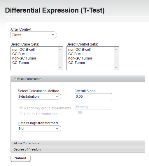
- Array Context - If more than one context for array sets has been created, first choose the desired context. Each context can contain its own collection of array sets. It is provided as a convenience.
- Select Case/Control Sets - In each of the two lists, select at least one array set. No array should be part of both case and control sets; if it is, the analysis will not be performed.
P-value Parameters
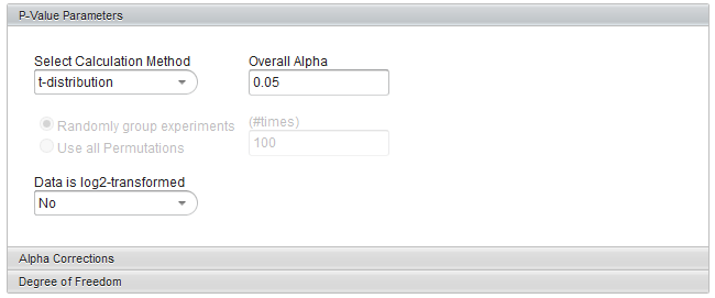
Select Calculation Method
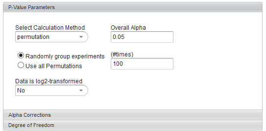
The p-values can be calculated by transforming the t-statistic directly, or by carrying out a permutation analysis. The permutation analysis measures how often a t-statistic at least as large as that observed occurs by chance after array labels of case and control are permuted.
- t-distribution (the default)
- Permutation - If chosen, the number of permutations to carry out must also be specified.
If permutation is chosen, the relevant controls become enabled
- Randomly group experiments Enter the integer number of random permutations to carry out in the adjoining text field (#times).
- Use all Permutatons - All possible permutations will be carried out.
Overall alpha (Critical p-value)
The threshold for a difference in expression between Case and Control sets being called significant (default 0.05). Multiple-testing corrections can be specified in the Alpha Corrections tab.
Data is log2-transformed
If the dataset has been Log2 transformed, select yes. Having this information allows the fold-change displayed in the Volcano Plot to be calculated in a consistent fashion.
Expression data typically better approximates a normal distribution if at has been log transformed. This can be performed in an external program such as geWorkbench desktop.
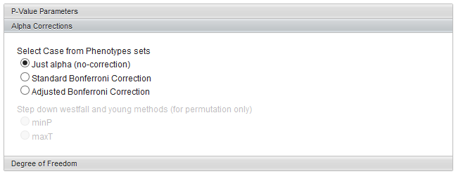
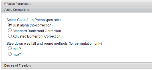
Alpha corrections
For multiple testing (alpha) correction with the standard t-distribution calculation, the following options are offered:
- Just alpha (no correction)
- Standard Bonferonni Correction - the value of alpha is divided by the number of markers included in the analysis.
- Adjusted (step down) Bonferonni Correction
If a permutation-based calculation method has been chosen, two variants of the Westfall and Young method also become available:
- minP
- maxT
Degrees of Freedom
Group variances can be declared as:
- unequal (Welch approximation) (default)
- Equal.
Example
Preparation
This example uses the file Bcell-100_log2.exp, which is the Bcell data described in the Tutorial_Data section, and which has been further normalized as follows:
- Threshold Normalization - set a minimum value of 1.0 for each data point,followed by
- Log2 transformation
You can also associate the Affymetrix HG-U95Av2 annotation file during data upload, although it is not required for this example. See the FAQ section for information on downloading the original annotation file from Affymetrix.
Set Parameters
- Array Context - "Class"
- Case array set - "GC-Tumor"
- Control array set - "GC B-cell"
- P-Value Parameters tab
- P-value Overall Alpha - 0.01
- Calculation method - t-distribution
- Data is log2 transformed - select "Yes"
- Alpha-corrections tab
- Standard Bonferroni
- Degree of Freedom tab
- Welch approximation - unequal group variances.
Running the t-test analysis
- Click Submit.
t-Test Results
Result Node
A t-test result node is placed into the Workspace as a child of the analyzed microarray dataset.
The list of significant markers is placed into a new set "Significant Genes" in Marker Sets. The number of markers in the set is shown in square brackets.
Fold Change
The method used to calculate fold change depends on whether the data was marked as log2 transformed or not during the t-test using the "Data is log2 transformed" box.
- Linear data ("Data is log2 transformed" box was not checked): the fold change is calculated, for each marker, as the Log2 transform of the average expression in the Case set divided by the average expression in the control set, that is,
Log2(Avg(cases)/Avg(controls))
or
Log2(Avg(cases)) - Log2(Avg(controls)).  (Difference of logs of averaged values).
- Log2 transformed data ("Data is log2 transformed" box was checked): In this case, for each marker, the average of the (log) case values minus the average of the (log) control values is calculated, that is,
Avg(cases) - Avg(controls). (Difference of averaged log values).
The fold change is not calculated if, for the linear case, the average case or control value is negative.
At present, in geWorkbench-web, the fold-change data is only available via the Volcano Plot visualizer.
Volcano Plot Visualizer
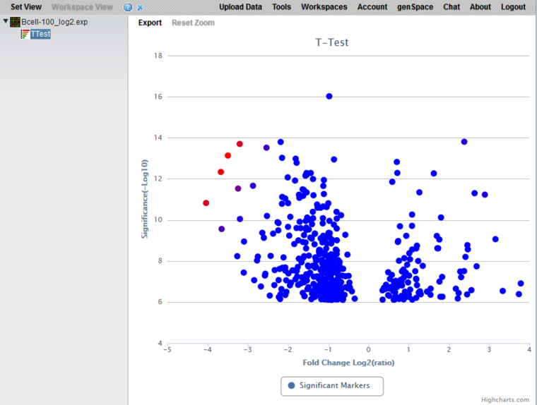
The Volcano Plot graphically depicts the results of the t-test for differential expression. It includes only markers which exceeded the threshold for significance in the t-test. The log2 fold change for each marker is plotted against -log10(P-value).
The fold change is calculate as described in the previous section based on whether the data was log2 transformed or not.
Color scheme
The lower 2/3 of the absolute values of the (fold change) * (significance) are colored in shades from light blue (lowest values) to dark blue (highest values). The highest 1/3 of such values are colored from dark blue (lowest values) to red (highest values).
- Note - the shading from light-blue to dark-blue is not currently working!
Hover text
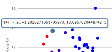
Hovering the cursor over a particular data point will highlight it as a larger blue circle and bring up a hover text displaying the marker name and its plot coordinates, the log2 fold change value and the -log10(p-value).
Export
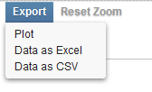
There are three export options:
- Plot - Open a SVG file in a new browser window.
- Data as Excel - Export the data to an Excel format file.
- Data as CSV - Export the data to a CSV format file.
For the Excel and CSV format files, the following colums will be contained in the file:
- Probe Set Name
- Gene Name (from Annotation file)
- p-Value
- Fold Change (Log2) - As calculated using one of the two methods described above.
Zoom and Reset Zoom
- Zoom action - The graph can be zoomed-in by left-clicking on the graph and dragging the mouse to select the zoom region.
- Reset Zoom - will return the plot to its original view.
