T-test
Overview
For the geWorkbench web version of T-Test please see T-Test_web.
A t-Test analysis can be used to identify markers with statistically significant differential expression between two sets of microarrays. In geWorkbench, these groups are specified as the "Case" and "Control" sets.
There are several steps to setting up a t-test analysis in geWorkbench.
- At least two sets of arrays must be available in the Arrays component.
- The array sets to be used in the analysis must be "activated" by checking the box adjacent to their names in the Arrays component.
- One or more activated array sets must be designated "Case", and the others "Control" (which is the default classification).
- The t-test parameters must be set.
After the t-test is run, the results will be displayed graphically, and all markers meeting the significance threshold are placed into a new Marker Set called "Significant Genes".
Please see the Example section below for instructions on preparing array sets for the t-test analysis.
As of geWorkbench 2.4.0, the t-test result is calculated using the Apache Commons Math Library.
t-Test Parameters
P-value Parameters
p-values based on
The p-values can be calculated by transforming the t-statistic directly, or by carrying out a permutation analysis. The permutation analysis measures how often a t-statistic at least as large as that observed occurs by chance after array labels of case and control are permuted.
- t-distribution (the default)
- Permutation - If chosen, the number of permutations to carry out must also be specified.
Overall alpha (Critical p-value)
The threshold for a difference in expression between Case and Control sets being called significant. A value of 0.05 is often used for a single test. Multiple-testing corrections can be specified in the Alpha Corrections tab.
Data is Log2-transformed
If the dataset has been Log2 transformed, check this box. Having this information allows the fold-change displayed in the Volcano Plot to be calculated in a consistent fashion.
The system will examine the current dataset and make a guess as to whether the data has been log2 transformed. The user can override this guess using the check box.
Alpha corrections
Several methods for correcting for the effects of performing multiple tests are offered, including Bonferroni and False Discovery Rate control. They differ in how they compare the calculated p-value to the cutoff value of alpha - the critical p-value for determining the significance of an observed difference.
- Just Alpha - No correction is performed.
- Standard Bonferroni - The cutoff value (alpha) is divided by the number of tests (genes) before being compared with the calculated p-values.
- Adjusted (step-down) Bonferroni - Similar to the Bonferroni correction, but for each successive P-value in a list of p-values sorted in increasing order, the divisor for alpha is decremented by one and then the result compared with the P-value. The effect is to slightly reduce the stringency (increase the power) of the Bonferroni correction. This is a step-down procedure.
- Two variants of the Westfall and Young method are available if the p-value is estimated by permuation:
- minP
- maxT
Degrees of Freedom
Group variances can be declared as:
- unequal (Welch approximation) (default)
- Equal.
Example
Preparation
This example uses the file Bcell-100.zip, which also is contained in the data/public_data directory of the geWorkbench distribution, and is further described in the tutorial data Tutorial_Data area. A version with the threshold normalizer and log2 transformations described below already applied is also available there.
You may also wish to load the Affymetrix HG-U95Av2 annotation file, although it is not required for this example. See the FAQ section for information on downloading this file from Affymetrix.
For tips on loading data files, see Local Data Files and Workspace.
In this example, we apply two normalization steps to the data set.
- Threshold Normalizer - set a minimum value of 1. Any value less than 1 will be set to 1.
- Log2 Transformation Normalizer - Log2 transform the data.
For an actual data analysis, you should apply data normalization steps appropriate to your own data and analysis design.
Array Classification
The t-test in geWorkbench requires that at least two sets of arrays be "activated". Only such "activated" sets are considered. In addition, at least one such set must be designated as "Case", and at least one other as "Control" (which is the default classification). Note that more than one set of arrays can be marked as "Case" or control.
Array set classification is covered in the Arrays/Phenotypes chapter. However, for convenience, the steps are illustrated here.
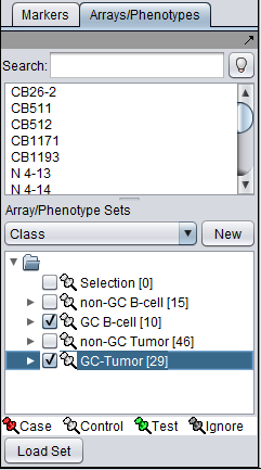
The desired sets of arrays should be activated in the Arrays/Phenotypes component. This is done by checking the boxes by the desired Sets.
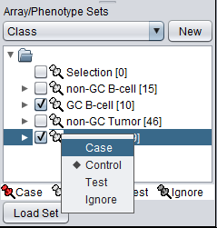
The classification can be made directly by left-clicking on the "thumb-tack" icon adjacent to an array set name.
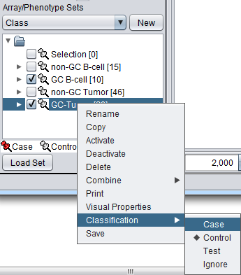
The array classification can also be set by right-clicking on the desired array set and selecting "Classification":
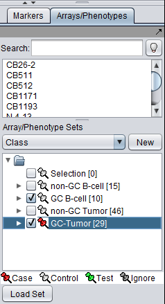
Using either method, the desired array set can be classified as "Case":
The thumbtack image next to activated Array Sets is colored red.
Setting the Analysis Parameters
- In this example, prior to the t-test, the BCell-100.exp data was threshold normalized to a minimum value of 1, then log2 normalized.
- The t-test component should be loaded by default in the Component Configuration Manager.
- From the Analysis Panel, select T-Test Analysis.
- P-value Parameters tab:
- P-values based on t-distribution.
- Note that here the default alpha (critical p-value) is set to 0.01.
- If the data has been log2 transformed, check-mark the box "Data is log2 Transformed".
- Alpha-corrections tab
- Standard Bonferonni
- Degree of Freedom tab
- Welch approximation - unequal group variances.
The P-value Parameters tab set for the example analysis:
Running the t-test analysis
- Click Analyze. The results will be returned in three locations: The Workspace, the Markers component, and the Visualization area.
t-Test Results
Result Sets
A t-test result node is placed into the Workspace as a child of the microarray dataset that was analyzed.
The list of significant markers is placed into a new set in the Markers component. This set is labeled "Significant Genes". The number in square brackets indicates the number of markers in the set.
Saving a Result Set
The result node (in the Workspace) can be saved by right-clicking on it and selecting "Save". This will save the significant markers in a CSV (comma separated value) file with the following columns:
- Probe Set Name
- Gene Name
- p-Value
- Fold Change (Log2)
Markers found significant in the t-test, but for which a fold change value could not be calculated, are included in the export file as "N/A".
Fold Change
The method used to calculate fold change depends on whether the data was marked as log2 transformed or not during the t-test using the "Data is log2 transformed" box.
- Linear data ("Data is log2 transformed" box was not checked): the fold change is calculated, for each marker, as the Log2 transform of the average expression in the Case set divided by the average expression in the control set, that is,
Log2(Avg(cases)/Avg(controls))
or
Log2(Avg(cases)) - Log2(Avg(controls)).  (Difference of logs of averaged values).
- Log2 transformed data ("Data is log2 transformed" box was checked): In this case, for each marker, the average of the (log) case values minus the average of the (log) control values is calculated, that is,
Avg(cases) - Avg(controls). (Difference of averaged log values).
The fold change is not calculated if, for the linear case, the average case or control value is negative.
Volcano Plot Visualizer
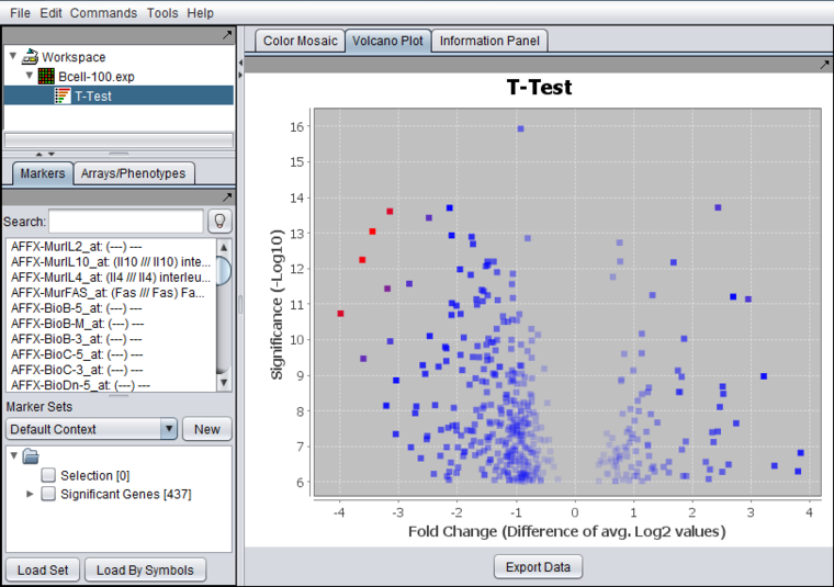
The Volcano Plot graphically depicts the results of the t-test for differential expression. It includes only markers which exceeded the threshold for significance in the t-test. The log2 fold change for each marker is plotted against the -log10 of the P-value.
Markers for which no valid fold-change value could be calculated (e.g. for the case of linear data the average of the case or control values was negative) are omitted from the Volcano Plot. However, all such markers are included if the data is exported to file.
See the Volcano Plot tutorial for further details.
Technical Notes
- If two data points have exactly the same coordinates, only the point which is "on top" will be shown when clicked-on or moused over.
- If the graph has only one point, or has several points all with the exact same coordinates, the default JFreeChart graphing behavior may omit a scale on the X or Y axis. The ranges of the axes and the labels can be manually adjusted. Right-click on the X or Y axis label area and select Properties->Range. Turn off "auto-ranging" and set the desired ranges.
Color Mosaic Visualizer
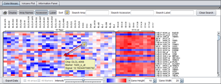
The Color Mosaic tab shows all arrays (or activated sets of arrays) and each significant marker with its p-value. By default, the markers are sorted by p-value. The display of each type of annotation can be switched on and off.
Please see the Color Mosaic tutorial for a complete description of all the features and controls of this viewer.
In the figure below, all display options have been activated, displaying array names at top, and p-value, accession (marker name), and gene name at left. The light-bulb indicates a hover text for the cell pointed to by the red arrow. The hover text displays the array (Chip) name, the marker name, and the signal value.


