SVM
Contents
Introduction
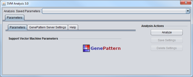
This component provides an interface to running the Support Vector Machines (SVM) algorithm on a GenePattern server. Documentation on the GenePattern implementation of SVM is available at GenePattern modules.
SVM is a supervised classification method that computes a maximal separating hyperplane between the expression vectors of different classes or phenotypes. Given microarray data with n markers per sample, SVM outputs a hyperplane,W, which can be thought of as a vector with n components each corresponding to the expression of a particular marker. Loosely speaking, assuming that the expression values of each marker have similar ranges, the absolute magnitude of each element in W determines its importance in classifying a sample.
In geWorkbench, the SVM computation compares one or more sets of arrays marked as "Case" against sets marked "Control".
The classifier that is generated can be applied to a test data set. This can be done in two ways. Before generating the classifier, additional arrays sets can be marked as "test". The new classifier will be applied immediately to the "test" data set. Or, after the classifier has been generated, "test" data nodes can be selected using a browser directly in the SVM component.
The result in either case is that the arrays in "test" set will be called as either belonging to the "Case" or "Control" categories, and a confidence value is indicated.
Parameters
The SVM module has no settable parameters for the computation.
GenePattern Server Settings
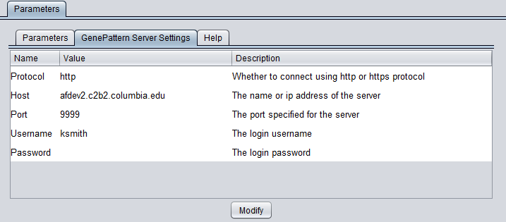
You can connect to any running GenePattern server to run the analysis (provided it has the required module installed). An example configuration of the "GenePattern Server Settings" tab is shown here:
To run GenePattern components, a GenePattern account is required.
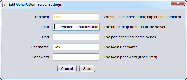
Pushing "Modify" brings up an editing box where any of the settings can be changed.
- Protocol - HTTP or HTTPS, depending on the server being used.
- Host - URL of a GenePattern server.
- Port - Port at which the GenePattern server is located on the Host machine.
- Username - A valid user name on the specified GenePattern server.
- Password - A password, if required by the specified server.
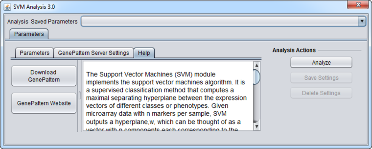
Help
GenePattern components in geWorkbench have their own brief built-in Help section.
Running an analysis
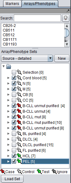
The SVM classifier requires that at least two sets of arrays be activated in the Arrays component. At least one must be marked as "Case" and at least one must be marked as "Control".
In addition, one or more additional sets can be activated an marked as "Test". After the classifier has been built using the "Case" and "Control" sets, it will be run on the "Test" set if one or more have been specified.
In the BCell-100 example dataset, we must first select the Arrays list "Source - detailed". From this list, we can select particular sets of arrays as shown below.
When "Analyze" is pushed, the data is transfered to the GenePattern server, and then the classifier will be run.
Training Classifier running:
Test classifier running:
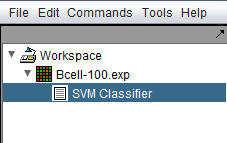
The resulting classifier is placed into the Workspace.
SVM Results Viewer
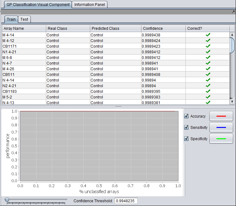
The SVM Results Viewer has three panes. "Train" (for training) and "Test" are viewed by selecting their tabs. The lower, graphical view applies to the classifier generated using the training data and is always visible.
Train tab
The training tab shows the results of applying the classifier to the original training data set. It has a tabular and graphical component.
- Array Name - each array included in the training data set is listed.
- Real Class - the classification as "Case" or "Control" in the training data set.
- Predicted Class - The predicted class resulting from applying the generated classifier to each array.
- Confidence - The confidence associated with the predicted class.
- Correct - Whether the predicted class agrees with the actual, known classification. A green check mark indicates agreement.
Graphical results display
The performance of the classifier (y-axis) is graphed against the percentage of unclassified arrays (x-axis). Three measures of performance are shown: Accuracy, Sensitivity and Specificity. The display of each may be enabled or disabled by toggling its check box. The color of the line representing each measure is shown adjacent.
- Confidence Threshold - The Confidence Threshold slider allows results to be filtered based on the confidence value. Only arrays with a confidence value exceeding the threshold are displayed in the table (and graph?).
The graphical results display shows the results for the generated classifier and is visible below both the "Train" and "Test" tabs.
Test tab
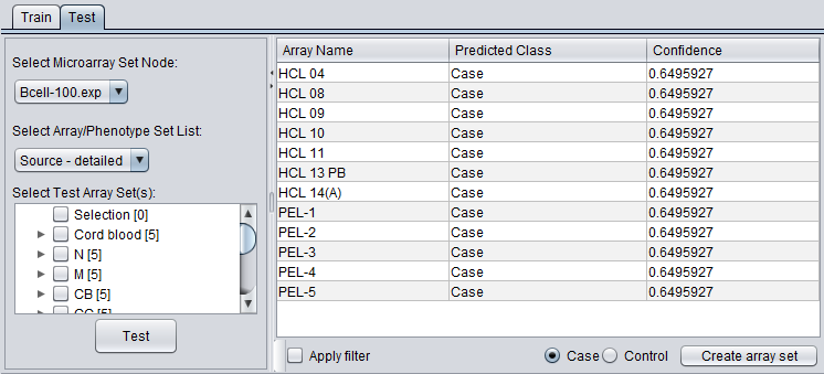
If one or more test sets were specified when the classifier was generated, the classification results fort the "test" set are shown in under the "Test" tab.
In addition, a data node browser allows array sets from any microarray data node to be selected. The classifier can then be applied to the selected array set.
Controls
- Select Microarray Set Node - Choose any microarray set present in the Workspace.
- Select Array/Phenotype Set List - Select a particular list of array sets available for the microarray set.
- Select Microaray Set - Select one or more tests array sets on which to run the classifier by marking the checkboxes next to their entry. If a set was already marked as a "test" set in the Arrays component, its entry will be automatically checked in this list.
- Test - Push the "test" button to begin the classification of the test data.
- Apply filter - If the check box is checked, the results in the tabular display will be limited to those arrays for which the confidence value exceeds the threshold set in the "Confidence Threshold" slider control underneath the graphical display.
- Create Array Set - Will create a new array set in the Arrays component containing the arrays classified as either the "Case" or "Control", depending on which of the adjacent radio buttons is selected.
- Case - create the new array set using the arrays classified as "Case".
- Control - create the new array set using the arrays classified as "Control".
Results
- Array Name - Each tested array is listed here.
- Predicted Class - The class to which each array was assigned by the classifier.
- Confidence - The confidence value for the assignment of the array to the class.
References - GenePattern
- Reich M, Liefeld T, Gould J, Lerner J, Tamayo P, Mesirov JP (2006) GenePattern 2.0 Nature Genetics 38 no. 5 (2006): pp500-501 doi:10.1038/ng0506-500. (PubMed 16642009)
- GenePattern website.
- GenePattern modules documentation.
References - SVM
- R. Rifkin, S. Mukherjee, P. Tamayo, S. Ramaswamy, C-H Yeang, M. Angelo, M. Reich, T. Poggio, E.S. Lander, T.R. Golub, J.P. Mesirov, An Analytical Method for Multiclass Molecular Cancer Classification, SIAM Review, 45:4, (2003).
- T. Evgeniou, M. Pontil, T. Poggio, Regularization networks and support vector machines, Adv. Comput. Math., 13 (2000), pp. 1-50.
- V. Vapnik, Statistical Learning Theory, Wiley, New York, 1998.
