geWorkbench

Overview

For the geWorkbench web version of ANOVA please see ANOVA_web.

The ANOVA (ANalysis of VAriance) algorithm (Zar, 1999) is used to determine whether any significant difference in the means exist in a dataset composed of three or more groups of experimental tests.

The geWorkbench ANOVA component implements a one-way analysis of variance calculation derived from TIGR's MeV (MultiExperiment Viewer) (Saeed, 2003). At least three groups of arrays must be specified by defining and activating them in the Arrays/Phenotypes component. For each chosen marker the routine determines if, at the specified level of significance, any difference in the mean exists in expression values between any of the groups (the null hypothesis is that there is no difference between the groups). Several basic methods of multiple testing correction are offered. The analysis does not indicate between which groups the difference is found, only that one exists.

Those markers for which a significant difference is found are placed into a new set in the Markers component called "Significant Genes". The results are also displayed in the Tabular Viewer and as a heat map in the Color Mosaic component.

Setting up an ANOVA run

Prerequisites

• To use the ANOVA routine, first check that it has been loaded in the Component Configuration Manager.
• At least three array sets must be already defined and activated in the Array Sets component.

ANOVA Parameters and Settings

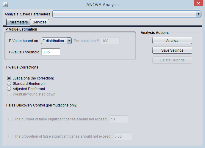
P-Value Estimation

The P-value represents, for any one test (one marker), the probability of falsely rejecting the null hypothesis - that is, calling a difference real when it is not. It is the probability that an F-statistic a least as large as obtained would be occur under the null hypothesis of no difference in means.

• P-value based on - Select one of two methods for calculating p-values:
  • F-Distribution - The p-value will be calculated using the F-distribution. The F-distribution arises from the ratio of the variances of two normally distributed statistics (chi-squared distributions).
  • Permutation - Permutations of the data will be used to generate a distribution against which the significance of the observed difference is judged. The number of desired permutations can be entered. The default number of permutations is 100.
• P-value threshold - sets the value of alpha, the critical p-value, for judging whether the null hypothesis can be rejected - that is, whether a difference is regarded as significant.

P-value corrections

Several methods for correcting for the effects of performing multiple tests are offered, including Bonferroni and False Discovery Rate control. They differ in how they compare the calculated p-value to the cutoff value of alpha - the critical p-value for determining the significance of an observed difference.

• Just Alpha - No correction is performed.
• Standard Bonferroni - The cutoff value (alpha) is divided by the number of tests (genes) before being compared with the calculated p-values.
• Adjusted (step-down) Bonferroni - Similar to the Bonferroni correction, but for each successive P-value in a list of p-values sorted in increasing order, the divisor for alpha is decremented by one and then the result compared with the P-value. The effect is to slightly reduce the stringency (increase the power) of the Bonferroni correction. This is a step-down procedure.
• Westfall-Young Step-Down - (Dudoit, 2003) Another step-down procedure which adjusts the critical value alpha using the Max T method. (This correction is only available when the permutation method is chosen for calculating p-values).

False Discovery Control

(This correction is only available when the permutation method is chosen for calculating p-values).

Rather than controlling the family-wise error rate (FWER) as do the Bonferroni corrections, that is, the probability of even one false positive occurring in the multiple trials, the false discovery rate calculation controls the rate of false positives. This can result in increased power to detect true differences. See Korn, 2001 and Korn, 2004, if one can accept more false positives. The number of false positives that is acceptable may be an economic decision, based on how many follow-up tests can be performed.

The user must select a limit to the rate of false discoveries as follows and enter the cutoff value in the adjacent text field:

• The number of false significant genes should not exceed - An upper limit on the number of false positives (markers falsely called as showing a significant difference), or
• The proportion of false significant genes should not exceed - An upper limit on the proportion of false positives.

Analysis Actions

• Analyze - start the ANOVA analysis
• Save Settings, Delete Settings - The geWorkbench analysis framework provides a standard method for saving one or more different sets of parameter settings per each type of analysis component. Please see the Analysis Framework Tutorial for further details.
  • Note - The False Discovery Control parameter fields will only have their values saved if they are actually selected. As they are controlled by radio buttons, only one text field can be active at one time, and hence only at most one of those fields will be saved in any one parameter set.

Services (Grid)

ANOVA can be run either locally within geWorkbench, or remotely as a grid job on caGrid. See the Grid Services section for further details on setting up a grid job.

Working with and Viewing ANOVA Results

Significant markers set

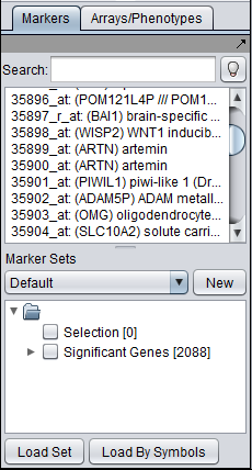
All markers which met the threshold p-value (alpha) cutoff are placed into the "Significant Genes" set in the Markers component. Such sets of markers can be used as the starting point for further characterization and analysis.

The ANOVA result node in the Workspace

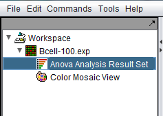
When the ANOVA calculation completes, the result node is placed in the Workspace. When the result node is selected (highlighted), the results will be displayed in both a tabular form and in the form of a heatmap in the Color Mosaic component.

Also shown is a "snapshot" node, that is a static picture of the heat map, labeled "Color Mosaic View". It was produced by right-clicking on the Color Mosaic display (see below) and selecting "Take Snapshot".

Color Mosaic Viewer

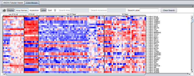
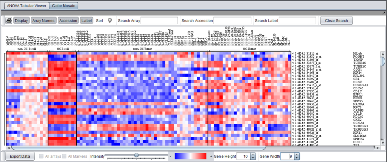
The Color Mosaic view displays the results as a heat map, which uses a color spectrum to indicate the relative magnitudes of the expression measurements. The heat map is colored using the currently selected color scheme (Menu->Tools->Preferences->Visualization). A color bar at the bottom shows the range of the color display and its correlation with expression values.

Columns represent individual arrays, and each row represents a marker. The arrays are grouped by the array set to which they belong, with each set labeled at the top of the picture. The markers are initially sorted in order of the calculated p-value, from smallest to largest. The p-values are shown at right in the diagram. Further details are available in the Color Mosaic tutorial.

The heat map depicted below was drawn using the "Relative" setting in the main Tools->Preferences->Visualization menu.

• Note - In the Color Mosaic display of ANOVA results, the "Sort" button has no effect. The "Sort" button is used only for the t-test, where it switches between ordering results by p-value and by fold-change.

Additional display options in the Color Mosaic view can be switched on to show array names and marker accession numbers (probeset ids):

Tabular Viewer

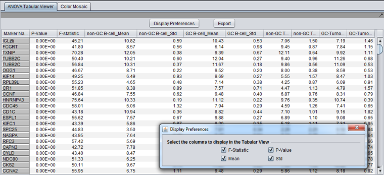
This Visual Area component displays a read-only spreadsheet view of the significant genes sorted by p-value in ascending order (from most significant to least significant).

Spreadsheet columns

• Marker Name - Shows the gene name if an annotation file has been loaded, otherwise shows the probeset name.
• F-statistic - the raw ANOVA score for each marker.
• P-value - the probability of observing an F-statistic this large by chance alone, assuming the null hypothesis of no actual differences between sets of arrays. If a multiple testing correction (e.g. Bonferroni) was used, the corrected p-value is reported.
• Mean - the mean expression value for each group of arrays.
• Std - the standard deviation for each group of arrays.

Controls

• Display Preferences - this button brings up a panel which controls which of the columns to display. The choices, described in the previous section, are F-statistic, p-value, mean, and standard deviation.
• Export - Click on Export in the lower left of the visualization to export this table in .csv format. The export file will contain only the columns displayed.

Further customizing the spreadsheet

• Resize columns by using the mouse to drag column boundaries.
• Reorder columns in the details pane by using the mouse to drag a column heading to the left or right of its original position.
• Sort the spreadsheet on a specific column by double clicking on its header. Succesive clicks will toggle between ascending order and descending order.

Dataset History

Details about each run are maintained in the Dataset History component. With the ANOVA result node highlighted in the Workspace, the Dataset History display includes the following information:

• P Value estimation method
• P Value threshold
• Multiple testing correction method
• Complete list of arrays in each group analyzed
• Complete list of all markers analyzed.

Example of running ANOVA

This example uses the Bcell-100.exp dataset available in the data/public_data directory of geWorkbench, and further described on the Download page. Briefly, this dataset is composed of 100 Affymetrix HG-U95Av2 arrays on which various B-cell lines, both normal and cancerous, were analyzed. Thus it explores a potentially wide variety of expression phenotypes.

Prerequisites

1. (Optional) Obtain the annotation file for the HG-U95Av2 array type from the Affymetrix NetAffx website (http://www.affymetrix.com/analysis/index.affx). The name will be similar to "HG_U95Av2.na34.annot.csv", where na34 is the version number. Loading the annotation file associates gene names and other information with the Affymetrix probeset IDs (see the geWorkbench FAQ for details on obtaining these files).

Loading and preparing the example data

1. Load the Bcell-100.exp dataset into geWorkbench as type "Affymetrix File Matrix". (See Local Data Files).
2. When prompted, and if desired, load the annotation file.
3. For this example, the data was subjected to threshold normalization with a minimum value of 1.0 followed by log2 normalization (See Normalization).

Choosing array groups

The Bcell-100 dataset comes with predefined sets of arrays.

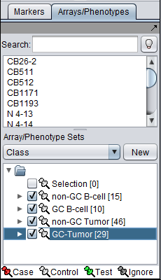
1. In the Arrays/Phenotypes component (at lower left in the geWorkbench GUI), choose the group in the pulldown menu called "Class".
2. Check the box beside each of the four sets of arrays to activate them as shown in the figure below.

Setting up the parameters and starting ANOVA

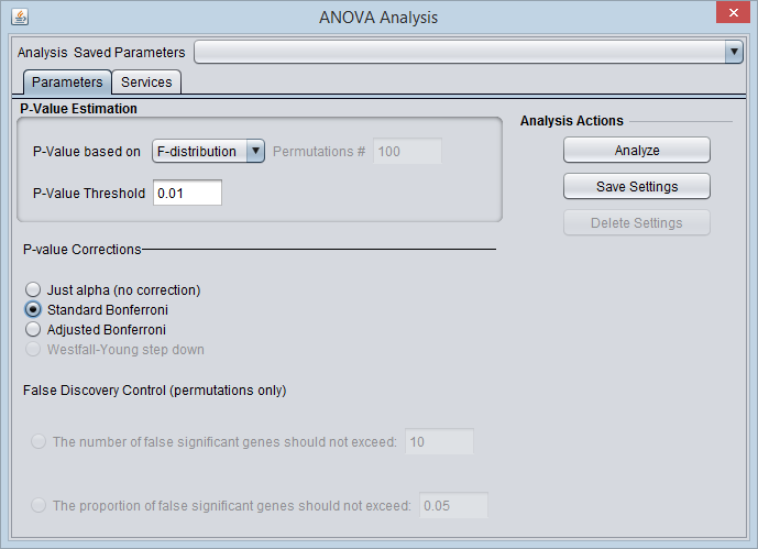
For this example we wil apply a relatively stringent multiple testing correction.

1. Leave the P-value method set to F-distribution.
2. Set the P-Value Threshold (alpha) to 0.01.
3. For the P-value correction choose Standard Bonferroni.
4. Push the Analyze button.

Results

The result of running ANOVA is a list of markers which meet the specified significance criteria. These markers are placed into a new set in the Markers component called "Significant Genes". The results are also displayed in visual components as detailed above for the Tabular Viewer and the Color Mosaic Viewer (Viewing ANOVA Results).

References

TIGR MeV lists the following relevant citations

• Dudoit S., J.P. Shaffer and J.C. Boldrick 2003. Multiple Hypothesis Testing in Microarray Experiments. Statistical Science 18: 71-103
• Korn, E.L., J.F. Troendle, L.M. McShane, R. Simon (2001).Controlling the number of false discoveries: application to high-dimensional genomic data. Technical report 003, Biometric Research Branch, National Cancer Institute. http://linus.nci.nih.gov/~brb/TechReport.htm
• Korn, E.L., J.F. Troendle, L.M. McShane, R. Simon (2004).Controlling the number of false discoveries: application to high-dimensional genomic data. Journal of Statistical Planning and Inference 124: 379-398.
• Saeed AI, Sharov V, White J, Li J, Liang W, Bhagabati N, Braisted J, Klapa M, Currier T, Thiagarajan M, Sturn A, Snuffin M, Rezantsev A, Popov D, Ryltsov A, Kostukovich E, Borisovsky I, Liu Z, Vinsavich A, Trush V, Quackenbush J. TM4: a free, open-source system for microarray data management and analysis. Biotechniques. 2003 Feb;34(2):374-8. PMID 12613259
• Zar, J.H. 1999. Biostatistical Analysis. 4th ed. Prentice Hall, NJ., pp 178-182.