Difference between revisions of "ANOVA"
(→Setting up an ANOVA run) |
(→P-value corrections) |
||
| Line 30: | Line 30: | ||
* '''Just Alpha''' - No correction is performed. | * '''Just Alpha''' - No correction is performed. | ||
* '''Standard Bonferroni''' - The cutoff value (alpha) is divided by the number of tests (genes) before being compared with the calculated p-values. | * '''Standard Bonferroni''' - The cutoff value (alpha) is divided by the number of tests (genes) before being compared with the calculated p-values. | ||
| − | * '''Adjusted Bonferroni''' - Similar to the Bonferroni correction, but for each successive P-value in | + | * '''Adjusted Bonferroni''' - Similar to the Bonferroni correction, but for each successive P-value in a list of p-values sorted in increasing order, the divisor for alpha is decremented by one and then the result compared with the P-value. The effect is to slightly reduce the stringency (increase the power) of the Bonferroni correction. This is a step-down procedure. |
| − | * '''Westfall-Young Step-Down''' - (This correction is only available when the permutation method is chosen for calculating p-values). | + | * '''Westfall-Young Step-Down''' - Another step-down procedure which adjusts the critical value alpha using a more complex expression. (This correction is only available when the permutation method is chosen for calculating p-values). |
| − | |||
===False Discovery Control=== | ===False Discovery Control=== | ||
Revision as of 15:55, 6 October 2009
Contents
Overview
The geWorkbench ANOVA component utilizes a one-way analysis of variance calculation from TIGR's MEV package. At least three groups of arrays must be specified by defining and activating them in the Arrays/Phenotypes component. For each chosen marker the routine determines if, at the specified level of significance, any difference exists in expression values between any of the groups (the null hypothesis is that there is no difference between the groups). Several basic methods of multiple testing correction are offered. The analysis does not indicate between which groups the difference is found, only that one exists.
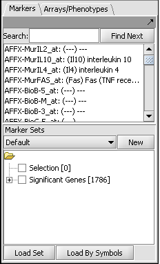
Those markers for which a significant difference is found are placed into a new set in the Markers component called "Significant Genes". The results are also display as a heat map in the Color Mosaic component.
Setting up an ANOVA run
Prerequisites
- To use the ANOVA routine, first check that it has been loaded in the Component Configuration Manager.
- ANOVA is found in the list of loaded analysis routines in the lower-right Commands quadrant of geWorkbench.
ANOVA Parameters and Settings
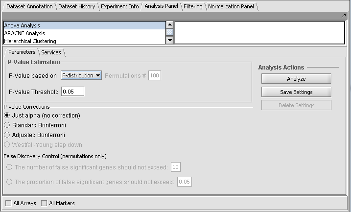
P-Value Estimation
The P-value represents, for any one test (one marker), the probability of falsely rejecting the null hypothesis by chance - that is, calling a difference real when it is not.
- P-value based on - Select one of two methods for calculating p-values:
- F-Distribution - The p-value will be calculated using the F-distribution. The F-distribution arises from the ratio of the variances of two normally distributed statistics (chi-squared distributions).
- Permutation - Permutations of the data will be used to generate a distribution against which the significance of the observed difference is judged. The number of desired permutations can be entered. The default number of permutations is 100.
- P-value threshold - sets the value of alpha, the critical p-value, for judging whether the null hypothesis can be rejected - that is, whether a difference is regarded as significant.
P-value corrections
Several methods for correcting for the effects of performing multiple tests are offered, including Bonferroni and False Discovery Rate control. They differ in how they compare the calculated p-value to the cutoff value of alpha - the critical p-value for determining the significance of an observed difference.
- Just Alpha - No correction is performed.
- Standard Bonferroni - The cutoff value (alpha) is divided by the number of tests (genes) before being compared with the calculated p-values.
- Adjusted Bonferroni - Similar to the Bonferroni correction, but for each successive P-value in a list of p-values sorted in increasing order, the divisor for alpha is decremented by one and then the result compared with the P-value. The effect is to slightly reduce the stringency (increase the power) of the Bonferroni correction. This is a step-down procedure.
- Westfall-Young Step-Down - Another step-down procedure which adjusts the critical value alpha using a more complex expression. (This correction is only available when the permutation method is chosen for calculating p-values).
False Discovery Control
(This correction is only available when the permutation method is chosen for calculating p-values).
The user must select the false discoveries in terms of either
- An upper limit on the number of false positives (markers falsely called as showing a significant difference), or
- An upper limit on the proportion of false positives.
Note on saving settings
The False Discovery Control parameter fields will only have their values saved if they are actually selected. As they are controlled by radio buttons, only one field can be active at one time, and hence only at most one of those fields will be saved in any one set.
Services (Grid)
ANOVA can be run either locally within geWorkbench, or remotely as a grid job on caGrid. See the Grid Services section for further details on setting up a grid job.
Viewing ANOVA Results
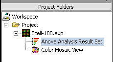
When the ANOVA calculation completes, the result node is placed in the Project Folders component. When the result node is selected (highlighted) in the project panel, the results will be displayed in both a tabular form and in the form of a heatmap in the Color Mosaic component.
Also shown is a "snapshot" node, that is a static picture of the heat map, labeled "Color Mosaic View". It was produced by right-clicking on the Color Mosaic display (see below) and selecting "Take Snapshot".
Color Mosaic Viewer
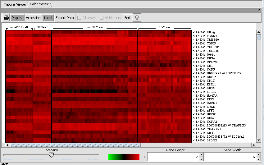
The Color Mosaic view displays the results as a heat map, which uses a color spectrum to indicate the relative magnitudes of the expression measurements. The heat map is colored using the currently selected color scheme (Menu->Tools->Preferences->Visualization). A color bar at the bottom shows the range of the color display and its correlation with expression values.
Columns represent individual arrays, and each row represents a marker. The arrays are grouped by the array set to which they belong, with each set labeled at the top of the picture. The markers are initially sorted in order of the calculated p-value, from smallest to largest. Further details are available in the Color Mosaic tutorial.
Tabular Viewer
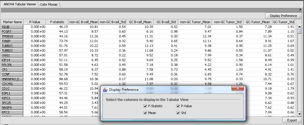
This Visual Area component displays a read-only spreadsheet view of the significant genes sorted by p-value in ascending order (from most significant to least significant).
Spreadsheet columns
- Marker Name - Shows the gene name if an annotation file has been loaded, otherwise shows the probeset name.
- F-statistic - the raw ANOVA score for each marker.
- P-value - the probability of observing an F-statistic this large by chance alone, assuming the null hypothesis of no actual differences between sets of arrays.
- Mean - the mean expression value for each group of arrays.
- Std - the standard deviation for each group of arrays.
Controls
- Display Preference - this button brings up a panel which controls which of the columns to display. The choices, described in the previous section, are F-statistic, p-value, mean, and standard deviation.
- Export - Click on Export in the lower left of the visualization to export this table in .csv format. The export file will contain only the columns displayed.
Further customizing the spreadsheet
- Resize columns by using the mouse to drag column boundaries.
- Reorder columns in the details pane by using the mouse to drag a column heading to the left or right of its original position.
- Sort the spreadsheet on a specific column by double clicking on its header. Succesive clicks will toggle between ascending order and descending order.
Significant markers set
All markers which met the threshold p-value (alpha) cutoff are placed into the "Significant Genes" set in the Markers component. Such sets of markers can be used as the starting point for further characterization and analysis.
Example of running ANOVA
This example uses the Bcell-100.zip dataset available and further described on the Download page. Briefly, this dataset is composed of 100 Affymetrix HG-U95Av2 arrays on which various B-cell lines, both normal and cancerous, were analyzed. Thus it explores a potentially wide variety of expression phenotypes.
Prerequisites
- Download and unzip the file Bcell-100.zip to obtain the Bcell-100.exp dataset.
- (Optional) Obtain the annotation file for the HG-U95Av2 array type from Affymetrix. The name will be similar to "HG_U95Av2.na29.annot.csv", where na29 is the version number. Loading the annotation file associates gene names and other information with the Affymetrix probeset IDs (see the geWorkbench FAQ for details on obtaining these files).
Loading and preparing the example data
- Load the Bcell-100.exp dataset into geWorkbench as type "Affymetrix File Matrix". (See from File).
- When prompted, and if desired, load the annotation file.
- For this example, the data was subjected to quantile normalization followed by log2 normalization (See Filtering and Normalizing.
Choosing array groups
The Bcell-100 dataset comes with predefined sets of arrays.
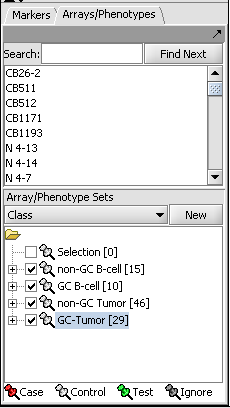
- In the Arrays/Phenotypes component (at lower left in the geWorkbench GUI), choose the group in the pulldown menu called "Class".
- Check the box beside each of the four sets of arrays to activate them as shown in the figure below.
Setting up the parameters and starting ANOVA
For this example we wil apply a relatively stringent multiple testing correction.
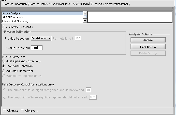
- Leave the P-value method set to F-distribution.
- Set the P-Value Threshold (alpha) to 0.01.
- For the P-value correction choose Standard Bonferroni.
- Push the Analyze button.
Results
The results are those shown in the figures in the previous section Viewing ANOVA Results.
