Difference between revisions of "SOM"
(→SOM Example) |
|||
| Line 5: | Line 5: | ||
==Limitations== | ==Limitations== | ||
| − | + | Version 1.03 of geWorkbench and earlier used an algorithm for Fast Hierarchical Clustering which does not implement the commonly understood versions of Average Linkage and Total Linkage. A standard version of these algorithms has now been implemented and will be included in the upcoming 1.04 release (expected August 18, 2006). Because we do not recommend use of the earlier algorithm, the tutorial will show results using the new implementation. The implementation of single linkage gives results as expected from the standard algorithm, but its use is in most cases not recommended due to its inherent poor properties with microarray data. | |
==Outline== | ==Outline== | ||
| Line 16: | Line 16: | ||
| − | == | + | ==Overview== |
Clustering methods can allow identification of groups of markers with similar expression. A common application is to search for genes that appear to be co-regulated. A list of such markers, saved to the '''Markers''' component, can be used for further steps, such as retrieving upstream sequences, Gene Ontology analysis, or viewing of annotations. | Clustering methods can allow identification of groups of markers with similar expression. A common application is to search for genes that appear to be co-regulated. A list of such markers, saved to the '''Markers''' component, can be used for further steps, such as retrieving upstream sequences, Gene Ontology analysis, or viewing of annotations. | ||
| − | |||
| − | |||
geWorkbench supports two clustering methods: | geWorkbench supports two clustering methods: | ||
| Line 58: | Line 56: | ||
==Hierarchical Clustering - Example== | ==Hierarchical Clustering - Example== | ||
| − | * Load the microarray dataset " | + | * Load the microarray dataset "webmatrix_quantile_log2_dev1.2_mv0.exp", available in the tutorial_data.zip [[Download]]. |
| − | * In the Arrays/Phenotypes component | + | * In this tutorial, we are going to include all arrays. |
| − | * | + | ** For a faster example, you could select subsets of arrays or markers in the Markers and Arrays/Phenotypes component. |
| − | * Go to the Analysis component, and select Hierarchical Clustering | + | ** You would do this by choosing a set in the pulldown menu there and checking the boxes in front of the desired subsets. |
| − | + | * Go to the Analysis component, and select Fast Hierarchical Clustering Analysis. | |
| − | |||
* In Hierarchical Clustering, set the parameters to: | * In Hierarchical Clustering, set the parameters to: | ||
** Clustering Method: Total Linkage | ** Clustering Method: Total Linkage | ||
| − | ** Clustering Dimension: | + | ** Clustering Dimension: Marker |
| − | ** Clustering Metric: | + | ** Clustering Metric: Pearson's |
*Click '''Analyze'''. | *Click '''Analyze'''. | ||
| − | The results | + | The results are placed in the Project Folders component and labeled "Hierarchical Clustering", and can be displayed in the Dendrogram component. |
| + | |||
| + | |||
| + | Here are results from using the previous implementation, and clustering on just two classes rather than all four: | ||
[[Image:T_HierarchicalClustering_BCregion.png]] | [[Image:T_HierarchicalClustering_BCregion.png]] | ||
Revision as of 19:00, 16 August 2006
Limitations
Version 1.03 of geWorkbench and earlier used an algorithm for Fast Hierarchical Clustering which does not implement the commonly understood versions of Average Linkage and Total Linkage. A standard version of these algorithms has now been implemented and will be included in the upcoming 1.04 release (expected August 18, 2006). Because we do not recommend use of the earlier algorithm, the tutorial will show results using the new implementation. The implementation of single linkage gives results as expected from the standard algorithm, but its use is in most cases not recommended due to its inherent poor properties with microarray data.
Outline
In this section the following information about clustering methods is covered:
- What clustering is and how it can be used.
- Methods implemented in geWorkbench: SOMs and Hierarchical Clustering
- An example of performing an SOM analysis
- An example of performing a Hierarchical Clustering analysis.
Overview
Clustering methods can allow identification of groups of markers with similar expression. A common application is to search for genes that appear to be co-regulated. A list of such markers, saved to the Markers component, can be used for further steps, such as retrieving upstream sequences, Gene Ontology analysis, or viewing of annotations.
geWorkbench supports two clustering methods:
- Self-Organizing maps (SOMs)
- Hierarchical Clustering
Self-organizing maps group the markers into a user-specified number of bins. In geWorkbench, a SOM visualizer component displays the results graphically. Hierarchical clustering constructs a tree-like relationship among the expression patterns of all markers present. Results are viewed in the Dendrogram component.
SOM Example
- Note - for the distance calculations used in SOM analysis to be valid, the data must have been normalized such that the scale of variation over each array is equal. (More details to be added here).
- Load the microarray dataset "webmatrix_quantile_log2_dev1_mv0.exp", available in the tutorial_data.zip Download.
- In the Arrays/Phenotypes component pulldown menu, select the group labeled "Class".
- Activate two sets of arrays to compare, e.g. GC B-cell and non-GC B-cell, by checking the boxes before the names (these are chosen here because they are the smallest groups).
- Go to the Analysis component, and select SOM Analysis.
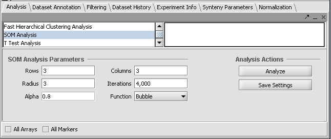
Parameters: Rows, Columns - give the number of bins into which to separate the different marker expression patterns. Radius - Iterations - Alpha - Function - Bubble or Gaussian
The default parameters are shown below. We will accept these parameters.
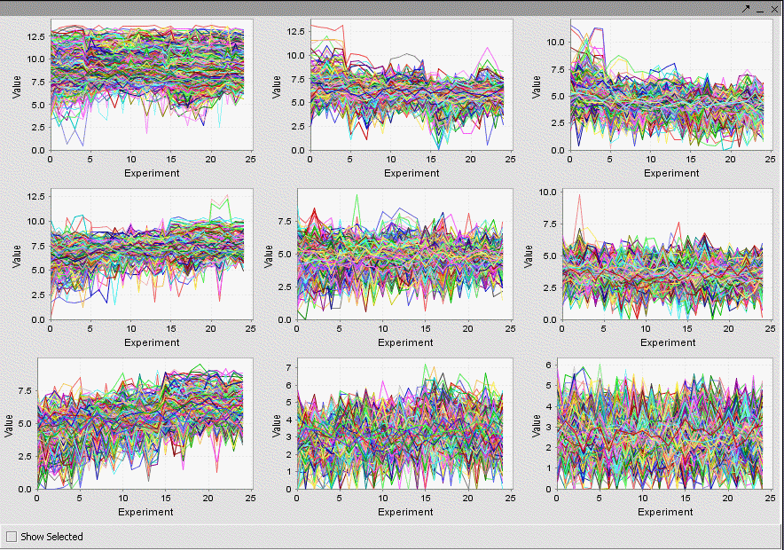
The resulting display of nine clusters is shown below. The user should experiment with different parameters to attempt to discern informative groupings.
Any individual graph can be right-clicked on and "Add to Set" chosen. This will add these markers to a new Set in the Markers component. Each will be given a name starting with "Cluster Grid" and the number of markers will be shown.
Hierarchical Clustering - Example
- Load the microarray dataset "webmatrix_quantile_log2_dev1.2_mv0.exp", available in the tutorial_data.zip Download.
- In this tutorial, we are going to include all arrays.
- For a faster example, you could select subsets of arrays or markers in the Markers and Arrays/Phenotypes component.
- You would do this by choosing a set in the pulldown menu there and checking the boxes in front of the desired subsets.
- Go to the Analysis component, and select Fast Hierarchical Clustering Analysis.
- In Hierarchical Clustering, set the parameters to:
- Clustering Method: Total Linkage
- Clustering Dimension: Marker
- Clustering Metric: Pearson's
- Click Analyze.
The results are placed in the Project Folders component and labeled "Hierarchical Clustering", and can be displayed in the Dendrogram component.
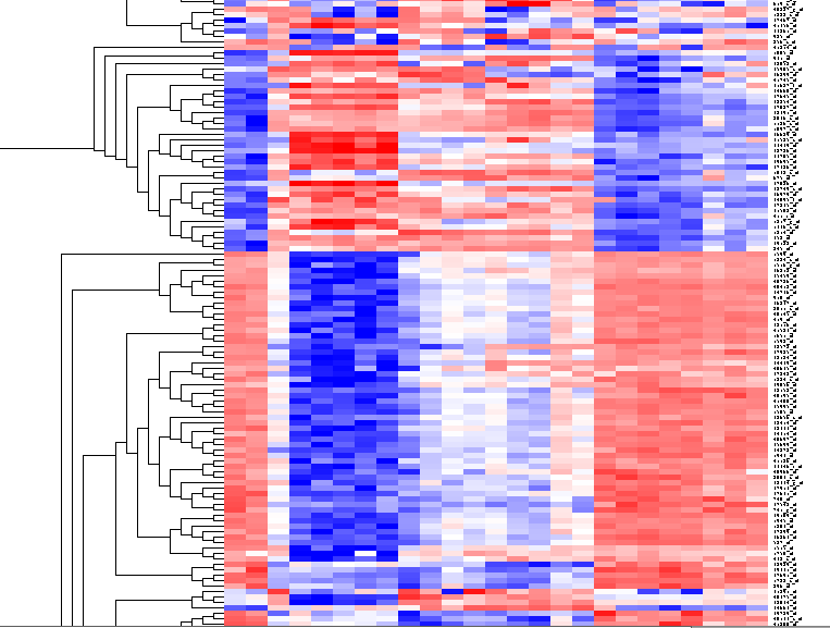
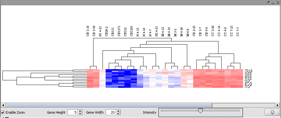
Here are results from using the previous implementation, and clustering on just two classes rather than all four:
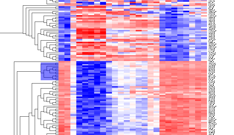
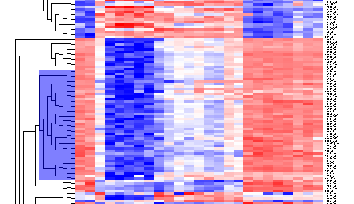
By scrolling down a bit, one finds a large interesting area, showing clear differences between groups of arrays. We will select two clearly differentiated clusters. Check the Enable Zoom checkbox. Then highlight the first cluster of 12 markers as shown here:
Then left-click to select this subset of the dendrogram. It will be displayed alone.
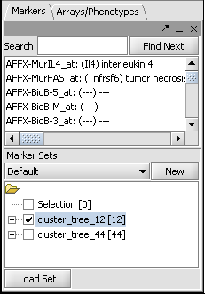
Now right-click and select "Add to Set". In the Markers component, the select genes are added as Cluster Tree [12], where 12 is the number of markers selected.
Repeat for the similar region just below, which contains another 44 markers.
This will result in two sets of markers having been added to the Markers component, as shown below:
