Overview

ARACNe (Algorithm for the Reconstruction of Accurate Cellular Networks) (Basso 2005, Margolin 2006a, 2006b) is an information-theoretic algorithm used to identify transcriptional interactions between gene products using microarray gene expression profile data. By proper selection of samples, a tissue (cellular context)-specific set of pairwise regulatory interactions (transcription factor-target) can be obtained – an “interactome”. Such an interactome can form the basis for more complex analysis of cellular regulatory networks. ARACNe has been used to reconstruct networks in mammalian cells for a number of specific tissue types.

For a dataset with a simple, monotonic relationship between input and output, analysis with a normal (e.g. Pearson's) correlation function may be the most suitable method. Where the input/output function is non-linear or irregular, a method based on the calculation of mutual information, such as ARACNe, may be able to find relationships that Pearson's correlation will not find. Calculation of the mutual information does not require a monotonic relationship. ARACNe has proven to be well suited for the reverse engineering of regulatory networks in the context of specific cellular types.

ARACNe performs best with a dataset containing data from a minimum of 100 microarrays (see Margolin, Wang et al. 2006) up to about 300-400 arrays, and representing a number of different states of the same cellular system - for example, cells lines of varying phenotype, or cells subjected to a variety of experimental perturbations. Initial work with ARACNe was performed using a large collection (about 340) of B-cell lines of various phenotypes (Basso et al. 2005). Note - For the "Fixed Bandwidth" option, using in excess of 300 arrays can lead to long computation times.

ARACNe can perform two separate calculations:

1. Mutual Information: The mutual information (MI) of one or more marker's expression profile(s) is calculated against all other markers.
2. Data Processing Inequality (DPI): The DPI calculation is used to remove the weakest interaction (edge) between any three markers. That is, if a MI value is available between each of three possible pairings of three markers, the weakest interaction of the three will be removed from the output. This has the intent of removing indirect interactions. For example, if A->B->C, the indirect interaction A->C will likely be weaker than A->B or B->C and would be removed. A tolerance can be set which relaxes this screening to account for uncertainty in the MI calculation.

Parameters described below allow one to incorporate a list of putative transcription factors and optimize the run to discover target genes that they may regulate.

Further information on ARACNe is available in the References section below.

Prerequisites

• A microarray dataset of sufficient size and phenotypic diversity is needed (See the Overview, above).
• Load the microarray dataset into the Workspace. A gene annotation file is not required for ARACNe, as it works at the probeset level. However, many other components of geWorkbench do require an annotation file be associated during upload.
• Warning on too few arrays - if a dataset with fewer than 100 microarrays is submitted for ARACNe analysis, a warning message will appear notifying the user of the suggested minimum of 100 arrays. Too few arrays may also cause the calculation to fail.

Parameters and Settings

Algorithm

Two algorithms are offered with which to calculate the pairwise mutual information between markers:

• Adaptive Partitioning (default) - fast calculation, and considered to produce superior results in certain circumstances.
• Fixed Bandwidth - previous, slower algorithm using a fixed Gaussian kernel. The kernel width parameter can be adjusted.

Mode

Choose whether to run the preprocessing calculation for a dataset, or to run ARACNe (Discovery mode)

• PREPROCESSING - Calculates dataset-specific parameters and stores them in "config" nodes in the workspace.
• DISCOVERY - Run the ARACNe mutual information calculation.

Preprocessing

In this mode, dataset-specific parameters are calculated. They are used to improve the mutual information calculation when Discovery mode is run. Preprocessing for a given combination of dataset and algorithm needs be run only once.

In general, preprocessing should always be run to improve the accuracy of the results. The only real exception is if you are running Adaptive Partioning with an MI value as the threshold, then pre-processing is not needed. Please be aware though that the raw MI values do not carry any information about their significance.

When running Discovery mode (below), if no preprocessing result node is specified, default parameters calculated from the B-cell dataset (see Margolin et al., 2006) are used as needed depending on the algorithm and options chosen.

• Fixed Bandwidth (FBW) algorithm - calculates parameters later used for (1) calculating the kernel width, and (2) for calculating a MI threshold from a specified P-value.
• Adaptive Partitioning (AP) algorithm - only the parameters used for calculating a MI threshold from a specified P-value are calculated. No kernel-width parameter is used.

Preprocessing parameter node names take the following form in the Workspace:

• "Aracne - AP - cfg22281": parameters for adaptive partioning. AP indicates this is a node for use (only) with adaptive partitioning. The job number is appended to "cfg".
• "Aracne - FB - cfg22282": parameters for fixed bandwith. FB indicates this is a node for use (only) with the fixed bandwidth method. The job number is appended to "cfg".

Please do not rename the nodes.

The parameters are displayed if the config node is clicked on, e.g.:

DISCOVERY

The ARACNe mutual information and the DPI (if selected) calculations are run.

Hub Marker(s) From Sets

The user must have already created a set of hub markers in the "Set View", either by selecting markers directly, or by uploading a list from a text file. Specifies which gene markers will be treated as "hubs" in the ARACNE mutual information (MI) calculation. The mutual information is calculated for each specified hub marker against all other markers in the submitted dataset. Typically, a list of known transcription factors is used to specify the hub markers. Such a list must be supplied by the user.

A pulldown menu allows selection from any marker set present (in the current marker context).

Threshold Type

Mutual Info.

Use the raw MI value calculated by ARACNe. Only interactions with MI above the threshold will be included in the final network. the MI can be any positive value or zero, but not negative.

P-Value

Use a p-value calculated from the MI values as the threshold. For best results, the preprocessing step must be run first to generate the parameters needed to calculate p-values from MI values for the particular data set.

Threshold

Enter the desired threshold value into the text field.

• Note - Using a P-value for the threshold is preferred to using the raw MI value, as the MI value conveys no information about significance.

Correction

If the threshold type is chosen as P-Value, an option to apply the Bonferroni multiple testing correction is offered in the adjacent pulldown menu.

• No Correction (default) - No correction is applied.
• Bonferroni Correction - Divide the specified p-value threshold by the (number of markers)*(number of hub genes tested).

Kernel width

The Kernel width is a scaling parameter used for fitting a Gaussian function to the data when running the FIXED_BANDWIDTH algorithm only, otherwise this field is disabled. If used, the value can be either inferred or specified directly.

• Inferred: If PREPROCESSING has been run on the dataset (mode is set to PREPROCESSING or COMPLETE), the kernel width is calculated directly from those results. If PREPROCESSING has not been run, the kernel width is inferred based on parameters fitted to a large B-cell dataset (Margolin et al, 2006), extrapolated for the number of samples in the dataset being tested.
• Specify: The user can enter a value for the kernel width directly, e.g. based on a prior calculation with this dataset.

DPI Tolerance

The Data Processing Inequality can be used to remove the effects of indirect interactions, e.g. if TF1->TF2->Target, DPI can be used to remove the indirect action of TF1 on the target. It is specifically intended to "remove indirect interactions mediated through two transcriptional interactions" (ARACNe Manual). The DPI tolerance specifies the degree of sampling error to be accepted, as with a finite sample size an exact value MI can not be calculated. The higher the tolerance specified, the fewer the edges that will be removed.

• Do Not Apply - Do not use the DPI.
• Apply (default) - In the text box, enter the fraction of the estimated MI to be considered as sampling error, expressed as a real number between 0.0 and 1.0. E.g. for 10%, enter 0.1. The default value of 0.0 (zero) is recommended.

For a full discussion of the theory and use of DPI in ARACNe, please see Margolin et al. (2006).

DPI Target List

The DPI Target List is used to give preference during application of the DPI to transcriptional interactions over those of genes that are e.g. tightly co-expressed but are not in a regulatory relationship to each other. An example of such co-expressed genes is genes for two proteins that are in a physical complex and hence always produced in the same amounts. If used, the DPI Target List should contain all markers that are annotated as transcription factors. Signaling proteins could also be included depending on the intended use of the network.

• Use of the DPI Target List prevents transcriptional interactions from being removed by non-transcriptional interactions when DPI is run.
• The DPI Target List comes into play when DPI examines a triangle of interactions which contains one TF and two non-TFs. If the weakest of the three interactions involves the TF (a TF-nonTF edge), then that edge would be removed by a simple application of the DPI. However, if the TF is included on the DPI Target List, the TF-nonTF edge will not be removed.

For further explanation and figures on the DPI Target list, see Chapter 3, note 7 of the ARACNe Manual.

• Do Not Apply - do not use a DPI target list.
• From Sets - select a marker set to use for the DPI target list. The marker set must have already been created in the "Set View".

Bootstrapping

Bootstrap analysis can be used to generate a more reliable estimate of statistical significance for the interactions. Please see Margolin et al. 2006, Nature Protocols, Vol 1, No. 2, pg. 663-672 for further details (full reference below). Briefly, repeated runs of ARACNE are made, with arrays drawn at random from the full dataset with replacement. The same number of arrays is drawn each time as is present in the original dataset. A permutation test is then used to obtain a null distribution, against which the statistical significance of support for each network edge connection (interaction) can be estimated.

• 100 rounds of Bootstrapping: (Checkbox) - when selected 100 rounds of bootstrapping are run in parallel on the C2B2 cluster.
• Consensus threshold (for bootstrapping only): After the bootstrapping runs are made, a permutation test is used to estimate the significance of interactions. The consensus threshold sets the cutoff point for calling the interactions significant and returning them in the final adjacency matrix

• Note - bootstrapping does not replace the need to filter the individual ARACNe runs using a p-value or MI threshold. That initial screening reduces the initial network to a tractable size, and is a prerequisite for the bootstrapping permutation step.

Merge multiple probesets

On a microarray analysis platform, genes may be represented by more than one marker (probeset). The mapping between markers and genes is specified in the annotation file, if it is read in at the time that the data is loaded. The ARACNe analysis in geWorkbench is performed at the level of probesets. In some cases, an interaction between two genes may be represented by more than one edge, each such edge involving an alternate probeset for at least one of the genes.

Selecting "merge multiple probesets" causes

• Yes - Merge multiple probesets. Interactions will be summarized at the gene level for each hub marker. The edge with the highest mutual information (MI) will be retained The resulting adjacency matrix will contain a single line per hub gene.
• No - Do not merge probesets. The full ARACNe adjacency matrix, as calculated at the probeset level, will be returned.

Analysis Actions

• Analyze - start the ARACNe analysis

Technical Note

• Multiple Gene IDs - In some cases, a marker may be annotated to more than one gene in the annotation file. Only the first such gene name on an annotation line is used when determining if two probesets map to the same gene.

Adjacency Matrix Result Node

The result of an ARACNe run is an adjacency matrix, placed as a new data node in the Workspace as a child of the microarray dataset from which it was generated. It contains the mutual information value for each pair of markers (or genes, if "merge probesets" was used) which exceeded the specified MI threshold. The adjacency matrix is placed into the Workspace as a child of the dataset that was analyzed.

The file format is described further in the File Formats chapter.

Viewing ARACNe results

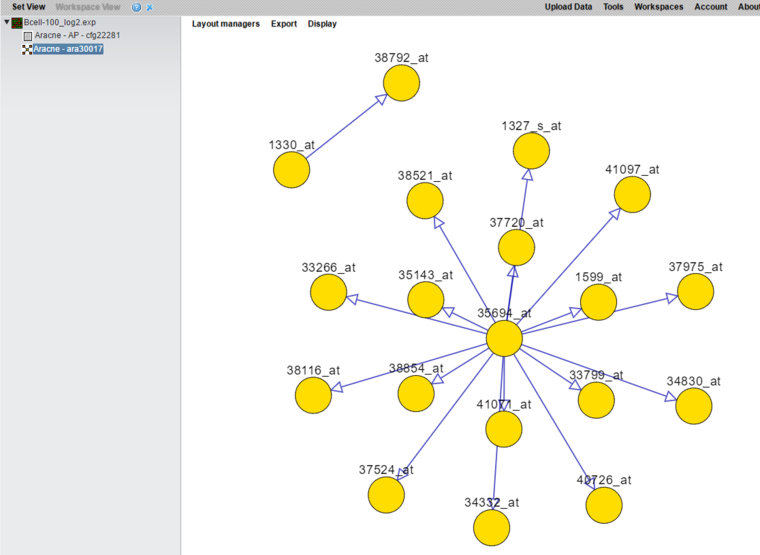
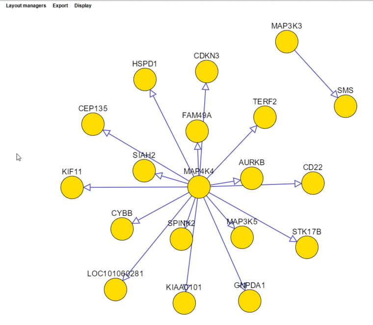
• The adjacency matrix can be visualized automatically in a viewer implemented using Cytoscape.js. Examples are shown below.

Dataset History

Details about each run are maintained in the Dataset History component. With the ARACNe result node highlighted in the Workspace, the Dataset History display includes the following information:

• Hub markers (list)
• Mode
• Preprocessing node used
• Algorithm
• MI threshold type and value
• Correction type
• DPI Tolerance usage and value
• DPI Target List usage
• Bootstrapping - number of bootstrapping runs (if > 1).
• Merge multiple probesets (yes/no)
• Count of markers in dataset
• Count of microarrays in dataset
• Timestamp

An example of the Dataset History, ommiting the lists of arrays and markers, is:

Aracne Parameters :

Hub Marker(s) from Sets - gc: 
 1476_s_at
 34715_at
Mode - Discovery
Configuration - Aracne - AP - cfg22281
Algorithm - Adaptive Partitioning
Threshold Type - P-Value: 0.01
Correction Type - Bonferroni Correction
DPI Tolerance - Apply  : 0.0
DPI Target List - Do Not Apply
100 Bootstrapping is not checked
Merge multiple probesets - No
Markers used (12600) - 
All Markers 
Phenotypes used (100) - 
All Arrays
Timestamp: Sep 23, 2016 3:51:52 PM

Example of running ARACNe and viewing results

This example uses the Bcell-100.exp dataset available in the data/public_data directory of geWorkbench, and further described on the Download page. Briefly, this dataset is composed of 100 Affymetrix HG-U95Av2 arrays on which various B-cell lines, both normal and cancerous, were analyzed. Thus it explores a potentially wide variety of expression phenotypes.

Prerequisites

1. (Optional) Obtain the annotation file for the HG-U95Av2 array type from the Affymetrix NetAffx website (http://www.affymetrix.com/analysis/index.affx). The name will be similar to "HG_U95Av2.na36.annot.csv", where na36 is the version number. Loading the annotation file associates gene names and other information with the Affymetrix probeset IDs (see the geWorkbench FAQ for details on obtaining these files).

2. Download the file Mapk_list.csv to your computer. These will be the hub markers.

Load Data

1. Load the Bcell-100.exp dataset into geWorkbench as type "Expression File (.exp)". (See Local Data Files).

2. If desired, load the annotation file. Loading the annotation file allows the resulting network to be expressed in terms of genes rather than probesets.

3. Switch to "Set View" and load the file "Mapk_list.csv" as a market set. It contains marker ids, not gene symbols.

Setting up the parameters and starting ARACNe

1. Switch back to Workspace view if you are still in "Set View".

2. In the Workspace, click on the expression file you just uploaded, BCell-100.exp.

3. At right, under the heading "Microarray Data", is the list of available commands. Click on ARACNe. You will see the parameter settings page.

Running Pre-processing

The pre-processing step is highly recommended to tune the ARACNe calculation to your dataset.

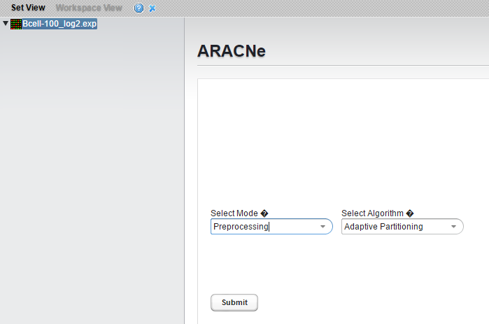
1. Select mode "Preprocessing" and algorithm "Adaptive Partitioning", and then hit "Submit". Note - this may take about 5 minutes to finish. (While "Preprocessing" mode is selected, you see only the choice for "Algorithm").

2. When preprocessing finishes, you will see a new "config" node appear in the Workspace as a child of the expression dataset you are analyzing.

Running Discovery

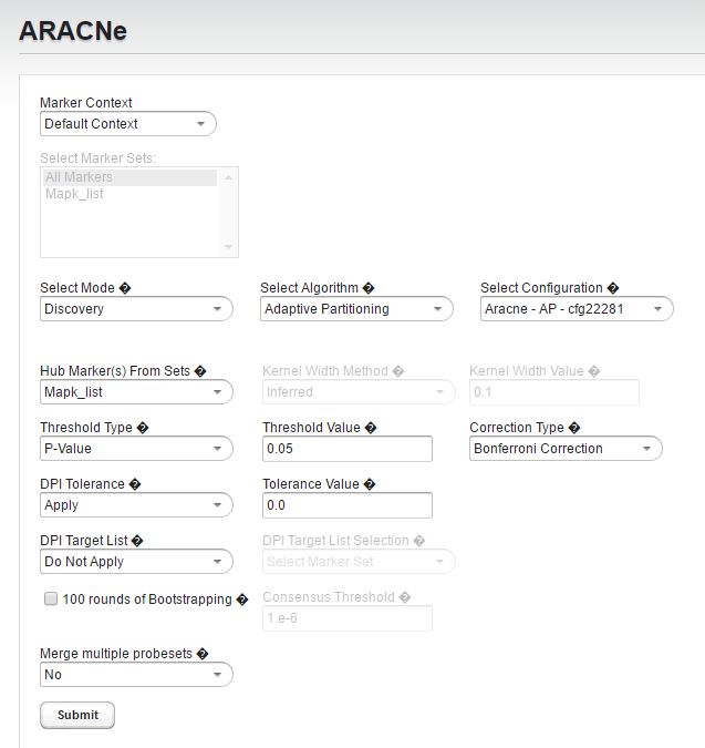
1. Select Mode: Discovery.

2. Specify Algorithm: Adaptive Partitioning. You will see the full parameter panel with all available settings.

3. Set Hub Markers From Sets to Mapk_list

4. Verify Threshold Type is P-value

5. Change Threshold Value to 0.05

6. Set Correction Type to Bonferroni

The full parameter list should now appear as follows:

• Mode: Discovery
• Algorithm: Adaptive Partitioning
• Hub Markers from Sets: Mapk_list
• Threshold Type: P-value
• Threshold Value: 0.05
• Correction: Bonferroni
• DPI Tolerance: Apply
• Tolerance Value: 0.0
• 100 rounds of Boostrapping - not checked
• Merge multiple probesets - No

5. Press Submit to launch the job. It should take only a few minutes.

6. The resulting network is shown below, drawn using Cytoscape.js.

Running Discovery with "Merge" enabled

This example is run just as above, but with the option Merge multiple probesets set to yes

• Merge multiple probesets - yes

Technical Notes

• Supplying the set of hub markers is the same as using the "-s" subnet option with the standalone ARACNe executable. "... a list of probes for which a subnetwork will be constructed".
• The DPI target list, if supplied, is the same as using the "-l" transcription factor option with the standalone ARACNe executable. "...a list of probes annotated as transcription factors in the input dataset".
  • "This option is ideal for transcriptional network reconstruction. If provided, DPI will not remove any connection of a transcription factor (TF) by connections between two probes not annotated as TFs. (However, this option has no effect if the list of hubs is already limited to transcription factors).
• If DPI is applied, the recommended tolerance value is now zero. In early publications, values up to 0.15 were recommended.
• When reconstructing transcriptional networks use of the bootstrapping option is recommended.
• Running with too few arrays can cause NaNs in Adaptive partioning preprocessing step, and in a NullPointerException in Fixed Bandwidth (Mantis issue 2030).
• The results of an ARACNe run depend to a small extent on the particular order of the arrays in the dataset - that is, reshuffling the arrays can give a numerically different MI.

References

• Basso K, Margolin AA, Stolovitzky G, Klein U, Dalla-Favera R, Califano A: Reverse engineering of regulatory networks in human B cells. Nat Genet 2005, 37(4):382-390. PMID 15778709, (link to paper).
• Margolin AA, Nemenman I, Basso K, Wiggins C, Stolovitzky G, Dalla Favera R and Califano A, (2006a) ARACNE: An Algorithm for the Reconstruction of Gene Regulatory Networks in a Mammalian Cellular Context, BMC Bioinformatics;7(Suppl.1):S7 (link to paper)
• Margolin A, Wang K, Lim WK, Kustagi M, Nemenman I, and Califano A (2006b) Reverse Engineering Cellular Networks. Nature Protocols 1(2):663-672 (link to paper)
  • Supplementary materials list
    • Supplementary materials - ARACNe Manual
    • Supplementary materials - Technical Report