geWorkbench

Overview

This chapter details the MARINa (MAster Regulator INference algorithm) method of Master Regulator Analysis. Please see the Master Regulator Analysis chapter for a higher-level introduction.

MARINa uses gene set enrichment analysis (GSEA) to calculate if the regulon of a TF is enriched for genes that are differentially expressed among 2 classes of microarrays. Please note that this does not involve any of the special gene lists available for use with the GSEA algorithm, such as MSigDB. Following the GSEA runs, MARINa performs an additional "shadow" analyses. The "Synergy" analysis option is not currently supported.

The MARINa algorithm runs on a computational cluster at Columbia and access is restricted. It is run from geWorkbench using a grid service, selected using the "Services" tab.

The MARINa algorithm differs substantially from the "FET" method described in the MRA-FET chapter.

1. The list of signature markers is determined using a t-test in the MARINa algorithm, rather than being loaded separately as for the FET method.
2. The list of candidate Master Regulators is taken from the network, rather than using a separate list as in the "FET" method.
3. The MARINa method has its own set of parameters.
4. MARINa will use case and control designations of arrays in the Arrays component if provided. However, unlike the FET method, it will also run if only control arrays are designated. This is a special case for use only where the loaded expression dataset has been pre-processed to represent fold-change values. geWorkbench itself cannot produce such a dataset.

A special 2-tailed version of GSEA is used, as described in Lim WK, Lyashenko E, Califano A (2009).

Inputs

Main Tab

These inputs and the GUI are described in detail in the chapter Master Regulator Analysis.

• Network - the network (e.g. from ARACNe) upon which MARINa will operate.
  • If the network is loaded into MARINa as gene symbols or Entrez IDs, it will be transformed (expanded) to include all probesets annotated to each such gene if an annotation file has been loaded for the expression dataset.
• GSEA P-Value: The enrichment score p-value below which a regulon is considered enriched in differentially expressed genes.

MARINa Tab

• GSEA and shadow/synergy analysis run parameters:
  • Minimum Number of Targets: minimum number of genes in a regulon for a GSEA run (a positive integer).
  • Minimum Number of Samples: minimum number of arrays PER CLASS (e.g. case or control) in the input microarray set in order to run sample-based permutations in GSEA (a positive integer). If sample-based permutations cannot be used, then probe shuffling will be used instead. The default is set to 6, but having a least 7 is better and 8 per class will give much better significance.
  • Number of GSEA permuations: number of GSEA permutations to compute enrichment score distribution (a positive integer).
  • GSEA Tail: whether 1-tailed (1) or 2-tailed GSEA (2) is to be performed. If all correlations in the network file are greater than zero, then one-tail GSEA will be performed regardless of the value the user assigns to "tail".
  • Shadow P-value: significance threshold for shadow analysis.
  • SynergyP-value: significance threshold for synergy analysis.
• Retrieve prior result with ID (checkbox) - if checked, all parameter fields are disabled and the prior ID field is enabled. The user can retrieve the results of a previous run. In this case, the "case" and "control" array sets do not need to be activated - they are retrieved from the MARINa run directory on the server.

GSEA Tail

If a two-tailed GSEA run is requested, the MARINa algorithm will divide a TF's regulon genes into positive and negative correlation groups, based on the Spearman's correlation between the expression of the TF and each gene in its regulon. However, if all correlations are found to be positive, only a single GSEA run will be performed. The correlation values are calculated by geWorkbench, or can also be provided directly if the "5-column network file" is used.

Sample Shuffling

Sample shuffling is done with random draws. If the number of samples per class is too low, the number of unique draws may be much lower than the number of permutations and lead to a false calculation of power.

The number of possible permutations is given by N!/2*{(N/2)!(N/2)!], where N is the total number of samples in the two classes together. The two in the divisor is because each draw of case and control arrays can occur in either order with identical result. That is, the two outcomes are not distinguishable in the calculation.

Note also that because random draws are performed, the number of unique draws will be less than the number of draws. If the number of samples per class is low, then many repeats of the same draw will be encountered.

For N=14 (that is, 7 per class), the number of unique results is 1716. For N=16 (8 per class), there are 6435 unique draws.

In addition, it is better if the number of samples per class is balanced, rather than say 6 in one class and 60 in the other class.

Finally, it is recommended to treat the calculated p-values with scepticism. One common correction is to multiply calculated p-values by a factor of 10, so a calculated p-value of 0.001 is treated instead as 0.01. This correction is not included in geWorkbench, but can be set by the user if so desired. That is, if you want a p-value of 0.01, instead set a p-value of 0.001.

Unpaired/Paired Runs

Normally, the user will specify two classes of arrays, e.g. "case" and "control". Under these conditions, an unpaired calculation is performed. However, if the user only includes one class of array (control), then "paired" analysis is performed. The assumption here is that the values are not direct expression values but are fold-change values for paired samples from patients. Such a pre-analyzed dataset would need to be loaded into geWorkbench, as there is no built-in method to performed such a paired analysis.

Network alternative 5-column file format

MARINa in geWorkbench will normally be set up to work with a network that is either already in the Workspace, or that is loaded from disk in a standard format, e.g. an ARACNe-style adjacency matrix or SIF file. geWorkbench will generate a file in the following 5-column format which is then sent to the remote MARINa service. However, a file in this format can also be directly loaded into the MARINa component. In this case, the values contained in the file are used directly, and are not replaced by values calculated by geWorkbench.

Each line represents a network edge and comprises five tab-delimited columns:

• Transcription factor id: A string that provides the transcription factor end of the edge. This is usually a probeset id or a gene symbol.
• Target id: A string that provides the target end of the edge. This is usually a probeset id or a gene symbol
• Mutual information: The mutual information (MI) of the edge (a real number). If the edge MI is not known/available, the value 1 can be entered here.
• Spearman's correlation: The Spearman's correlation for the edge, computed on the original microarray set that gave rise to the ARACNe network (a real number). If not known/available, the value 1 can be entered here.
• P-value for Spearman's correlation. The p-value associated with Spearman's correlation found in the previous column (a real number between 0 and 1). It this p-value is not known/available, a value of 0 can be entered here.

Example data files for running MARINa

MARINa runs, even on a large computational cluster, can be very time-consuming. We include here a small test dataset with which to demonstrate running MARINa.

Example data files (.zip). Includes expression file, network file (5-column format) and files defining two microarray classes. The individual files are:

• mra_grid_data.exp - Affymetrix File Matrix format expression file.
• mra_grid_5colnetwork.txt - A network file matching the expression data. This file is in the "5-column" format and can only be loaded directly into the MRA component. Network files in the adjacency matrix and SIF formats should normally be used, this file is for demonstration only.
• mra_grid_ixclass1.csv - array set definition file, for loading into the Arrays component to define phenotype class 1 (Case).
• mra_grid_ixclass2.csv - array set definition file, for loading into the Arrays component to define phenotype class 2 (Control).

Running MARINa

Prerequisites

• Expression Data
  • An expression data set must be loaded in geWorkbench.
  • The expression data should be log transformed for best results with the t-test.
• Phenotypic classes - specified in the Arrays component in the currently active list view.
  • Two classes - Normally, "case" (reported as class1) and "control" (reported as class2) array sets should be defined and activated in the Arrays component. There can be no arrays that belong to both classes. If there are, a warning will be displayed and the analysis will not be launched. With two specified classes, the calculation will be run in "unpaired" mode.
  • Single class - However, if only one class is present (e.g. if no arrays are marked "case" or activated, then only a single class will be used. In this case, the calculation is run in "paired" mode. This mode assumes that the expression data already represents fold-change results, a type of data manipulation that is not directly supported in geWorkbench. This data should be either e.g. log2(case/control) or log2(case) - log2(control).
• Network file - a network that is already present in the Workspace as a child of the expression dataset can be used, or a network can be loaded directly into the MRA component via its Main tab.

Setting the MARINa Parameters

Please note that MARINa analysis can only be selected in the Services tab as a grid service. Just opening the MARINa parameters tab does not select the MARINa service.

Main Tab

• In the Main tab of the MRA component, select or load a network.
• Set the desired GSEA p-value.

Please see the description of this tab in the Master Regulator Analysis chapter.

Selecting the MARINa grid service

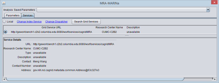
• You must search for and activate the MARINa grid service in the MRA services tab. If the local service is selected it will run the FET method.

The figure below shows the Services tab after the MARINa grid service has been retrieved and selected.

MARINa Tab

• Inspect and if desired change the parameters. See the section on "Inputs" above.

Analyze

Push the Analyze button to launch the analysis on the grid service. You will be prompted to enter a grid username and password.

Results

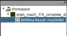
The MARINa calculation result is placed in the Workspace as a new data node. The name of the node takes the form "MARINa Result: mranum, where num is a job id assigned on the server.

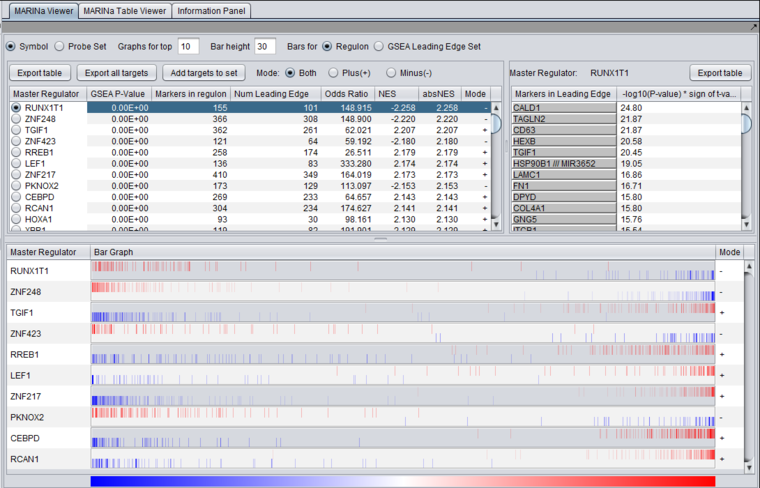
Results Viewer

Table Viewer

This example was run with sample shuffling. When probe shuffling is used, the MeanClass1 and MeanClass2 columns are not shown.

The MARINa results file contains one line for each TF whose GSEA enrichment score renders it significant above the user-specified p-value threshold (pvalue_gsea), as long as such TF is not "shadowed" by other significant TFs. NOTE: for the time being, we will ignore below (and in our implementation of the grid service) the results of the synergy analysis.

The columns represented in the results are as follows:

• TFsym: transcription factor id (usually this is the probeset id).
• GeneName: transcription factor gene name.
• NumPosGSet: number of genes (among those in the regulon of the transcription factor) which are positively regulated by the TF. Only genes represented in the microarray set are counted.
• NumNegGSet: number of genes (among those in the regulon of the transcription factor) which are negatively regulated by the TF. Only genes represented in the microarray set are counted.
• NumLedgePos: number of genes (among those counted under the NumPosGSet column) which are in the GSEA leading edge.
• NumLedgeNeg: number of genes (among those counted under the NumNegGSet column) which are in the GSEA leading edge.
• NumLedge: sum of NumLedgePos and NumLedgeNeg.
• ES: GSEA enrichment score for the regulon of the TF.
• NES: GSEA normalized enrichment score for the regulon of the TF.
• absNES: absolute value of NES
• PV: p-value of normalized (?) enrichment score.
• OddRatio: odds of a regulon gene being in the GSEA leading edge set / odds of a regulon gene being in the GSEA trailing edge set.
• TScore - t-test t-statistic.
• MeanClass1: mean expression value of TF among all "Class 1" arrays.
• MeanClass2: mean expression value of TF among all "Class 2" arrays.
• Note - there are no MeanClass1 and MeanClass2 when probe shuffling is performed.
• Original MRA/Recovered_MRA: a value of 1 in this column means that the TF was found to be enriched by GSEA (above the significance level pvalue_gsea) and that it was not shadowed by any other TF. A value of 0 means that the TF was found to be enriched by GSEA and that it was shadowed by another TF and that it remained enriched even after the common targets with the other TF were removed from its regulon. For details on Shadow analysis please see pg. 17 of the Supplemental text to Lefebvre et al. 2010..

References

• Basso K, Margolin AA, Stolovitzky G, Klein U, Dalla-Favera R, Califano A (2005). Reverse engineering of regulatory networks in human B cells. Nat Genet 37(4):382-390 (link to paper).

• Carro MS, Lim WK, Alvarez MJ, Bollo RJ, Zhao X, Snyder EY, Sulman EP, Anne SL, Doetsch F, Colman H, Lasorella A, Aldape K, Califano A, Iavarone A (2010) The transcriptional network for mesenchymal transformation of brain tumors. Nature 463(7279):318-25.
• Lefebvre C, Rajbhandari P, Alvarez MJ, Bandaru P, Lim WK, Sato M, Wang K, Sumazin P, Kustagi M, Bisikirska BC, Basso K, Beltrao P, Krogan N, Gautier J, Dalla-Favera R, Califano A (2010) A human B-cell interactome identifies MYB and FOXM1 as master regulators of proliferation in germinal centers. Mol Syst Biol. 6:377. PMID: 20531406 (link to paper).

• Lim WK, Lyashenko E, Califano A (2009) Master regulators used as breast cancer metastasis classifier. Pac Symp Biocomput. 2009:504-15. PMID 19209726, (link to paper).