geWorkbench

Preparation: An example of filtering and normalization

The file "webmatrix.exp" contains results from 100 Affymetrix HG-U95Av2 chips containing B-cell samples from numerous different disease states (phenotypes). 12600 markers are represented. To prepare this dataset for clustering we will filter and normalize the data. The steps shown are just an example of how filtering and normalization can be used, and each dataset should be handled according to the type of analysis being undertaken and its goals.

For this dataset, we performed the following steps:

1. Applied Expression Threshold Filter to remove very low expression values in the range 0-20.

2. Applied the Missing Values Filter with a maximum number of missing values per marker of 2. (Deletes markers with more than 2 missing values). This reduced the number of markers to 6327.

3. Performed Quantile Normalization using Averaging Method of Mean Marker Profile.

4. Applied the Deviation Filter with Deviation Bound of 20 and Missing Values set to Marker Average.

5. Applied the Missing Values Filter as in (2), which further reduced the number of markers to 6270.

The resulting dataset was named webmatrix_fn.exp.

Fast Hierarchical Clustering

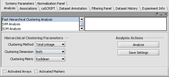
Fast Hierarchical Clustering is found in the Analysis Panel.

In this example we shown Hierarchical Clustering being performed with the following options:

1. Clustering Method: "Total Linkage"

2. Clustering Dimension: "Both"

3. Clustering Metric: "Euclidean"

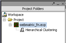
Hit Analyze to run the clustering. The resulting dataset is inserted into the Project Panel

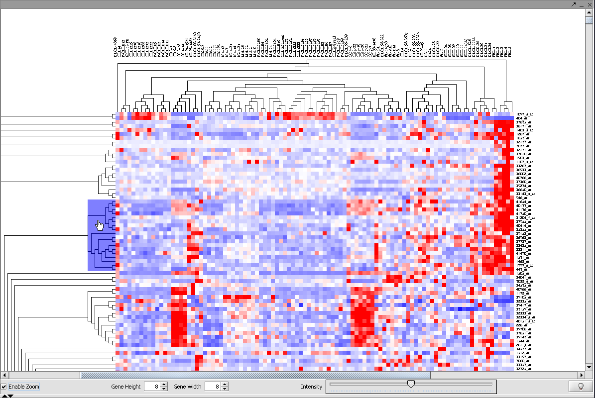
and can be viewed in Dendrogram.

Selecting a subtree in Dendrogram

Here we will pick a subtree near the top for further investigation.

1. Click Enable Zoom.

2. Position the mouse pointer over the cluster subtree of interest. It will be highlighted in blue.

3. Left-click on the highlighted subtree to view it alone.

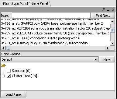
4. By right-clicking on the image, and selecting "Add to set",

(note that the picture uses a previous notation, "Add to Panel"

the markers in this subtree can be added as a new marker set in Markers. It will be given the default name "Cluster Tree".