SOM
Contents
Overview
The SOM (Self-Organizing Maps) method clusters markers into a user-specified number of bins based on their similarity to each other. In geWorkbench, a SOM visualizer component displays the results graphically. The markers clustered into a particular bin can be saved as a set back to the Markers component for further analysis.
- Note - for the distance calculations used in SOM analysis to be valid, the data should be normalized such that the scale of variation over each array is equal.
SOM Parameters
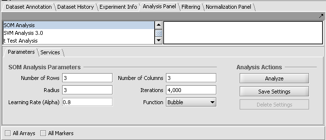
Number of Rows and Columns
The final graphical display will be laid out using the given number of rows and columns. The product of the two gives the number of bins into which the markers will be clustered. Both rows and columns must be greater than 0.
Radius
When using the bubble neighborhood parameter this float value is used to define the extent of the neighborhood. If an SOM vector is within this distance from the winning node (the cluster to which an element has been assigned) then that Node (and SOM vector) is considered to be in the neighborhood and its SOM vector is adapted. This must be a number greater than 0.
Iterations
The number of times the dataset will be presented to the Map. Each expression element will be presented this number of times to train the Nodes. This must be a number be greater than 0.
Alpha
This value is used to scale the change of individual SOM vectors when a new expression vector is associated with a node. This must be a value between 1 and 0.
Function
The neighborhood options indicate the conventions (formulas) used to update (adapt) an SOM vector once an expression vector has been added into a Node's neighborhood.
Bubble
This option uses the provided radius (see above) to determine which surrounding SOM nodes are in the neighborhood and therefore are candidates for adaptation. When this option is selected the Alpha parameter for scaling the adaptation is used directly as provided from the user.
Gaussian
This option forces all SOM vectors in the network to be adapted regardless of proximity to the winning node. In this case the Alpha parameter is scaled based on the distance between the SOM vector to be adapted and the winning node's SOM vector.
Service
The Service subtab allows the user to select which compute server to use to run the analysis: Local or Grid. The local instance of the server runs on the user's machine; GRID allows the user to pick up one among the available caGrid-enabled versions of SOM Clustering.
Analysis Actions
Analyze
Populate the parameters of the analysis and click on Analyze. The results are displayed in the SOM Clusters visualization component.
Save Settings
Save the current settings for this analysis component.
Delete Settings
Delete the currently highlighted set of saved parameters.
SOM Example
For this example we will start with the data set used in the ANOVA tutorial. Briefly, the Bcell-100.exp dataset was quantile normalized and log2 transformed. A set of markers found by ANOVA analysis of four groups of arrays was saved to the Markers component. It is this set of markers which will here be clustered.
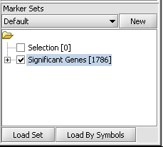
1. If desired, select a subset of markers and/or arrays on which to cluster. The following figure shows the set of 1786 markers found in the ANOVA example has been activated by checking the adjacent check-box.
2. Set the SOM parameters. The default parameters are shown above in the Parameters section. We will accept these parameters.
3. Push Analyze. The result will be displayed graphically in the SOM Clusters Viewer.
4. The user might experiment with different parameter settings to attempt to discern informative groupings.
SOM Clusters Viewer
Show selected
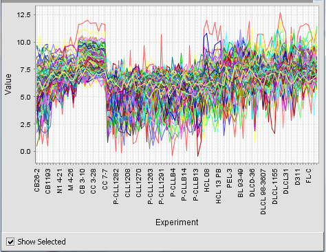
If the "Show selected" box is checked, the user may then click on any of the clusters and it will be enlarged to fill the display area. Unchecking the "Show selected" box will return to the original display of all clusters.
Left-click action
When a point on a cluster is clicked on with the mouse, the marker and array it corresponds to will be hightlighted in the Markers and Arrays/Phenotypes components, respectively.
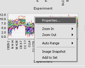
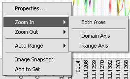
Right-clicking on a cluster produces the menu shown below.
The individual choices are:
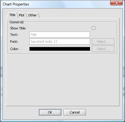
Properties Zoom In/Zoom Out Auto Range Image Snapshot Add to Set
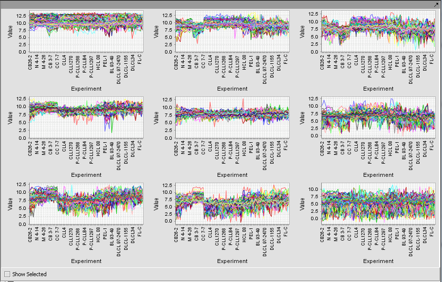
Running the example just described, with 3 rows and 3 columns, produces the nine clusters shown below.
Any individual graph can be right-clicked on and "Add to Set" chosen. This will add these markers to a new Set in the Markers component. Each will be given a name starting with "Cluster Grid" and the number of markers will be shown.
Saving the list of genes
For use in future examples, you can save a list of genes from the Markers panel:
- Highlight its entry in the Markers component (Cluster Tree[84]).
- Right-click and select "Save".
- Enter a name. We have saved the list from the above hierarchical clustering example as "cluster_tree_total_pearsons_84_markers.csv". (The .csv is added automatically). This list is available under this name in the tutorial data download.
