geWorkbench

Overview

geWorkbench implements its own code for agglomerative hierarchical clustering. Starting from individual points (the leaves of the tree), nearest neighbors are found for individual points, and then for groups of points, at each step building up a branched structure that converges toward a root that contains all points. The resulting graph tends to group similar items together.

Setting up

A microarray dataset must be loaded in the Project Folders component.

Note - hierarchical clustering is memory intensive. With the default memory settings (see here to change), clustering more than about 2000 markers is not recommended.

Missing Values

If there are any missing values in the dataset, an error message will be returned if Hierarchical Clustering is run. Missing values can be filtered out or replaced using the Missing Value Filter or the Missing Value Normalizer.

Parameters

Clustering Method

Specifies the method used to measure the distance between two clusters as the hierarchical tree is constructed. In each, the distance from each point in one cluster to each point in a second cluster is calculated, giving a set of pairwise distances. The methods differ in how the overall distance between the clusters is measured:

Single Linkage

The smallest pairwise distance found between the two clusters is used.

This method often leads to a "chaining" effect and is usually not recommended.

Average Linkage

The average of all the pairwise distances between the two clusters is used.

Total Linkage

The largest pairwise distance found between the two clusters is used.

Clustering Dimension

Marker

Cluster the selected markers (genes) only based on the similarity across selected microarrays.

Microarray

Cluster the selected microarrays only based on the similarity across selected markers.

Both

Cluster both markers and microarrays.

Clustering Metric

The values being clustered, whether markers or microarrays, can each be represented by vectors of numbers, essentially either rows (markers) or columns (microarrays) taken from a spreadsheet view of all expression values. Several methods by which to calculate the distance between any two vectors are offered:

Euclidean

The direct, point-to-point distance is calculated (square root of the sum of square differences).

Pearson's

Pearson's correlation coefficient for two vectors is calculated.

Spearman's

Spearman's rank correlation coefficient for two vectors is calculated.

Set Selection

Most geWorkbench analysis components provide the "All Arrays" and "All Markers" check-boxes to allow any activated sets of arrays or markers to be overridden. Normally, activating one or more sets of markers or arrays limits an analysis to those items in the active set(s).

All Arrays

Use all arrays in the dataset.

All Markers

Use all markers in the dataset.

Services

Several geWorkbench analysis routines have been implemented as analytical services available on caGrid. On the services tab, the user can select whether to run a job locally or using a grid service.

Example

Running the calculation

This example will take off with the set of markers produced in the ANOVA example. Please follow the steps for that example to produce the starting marker set, or just create/select another set of markers of your own.

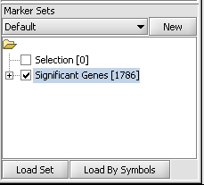
1. If following the ANOVA example, activate the set of markers labeled "Significant Genes [1786]" ( which contains 1786 markers).

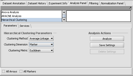
2. Set the parameters as shown in the following figure.

• Clustering methods: Average Linkage.
• Clustering Dimension: Marker.
• Clustering Metric: Euclidean.

3. Click Analyze.

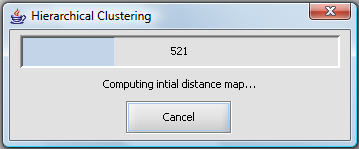
4. A progress bar will be visible during the calculation.

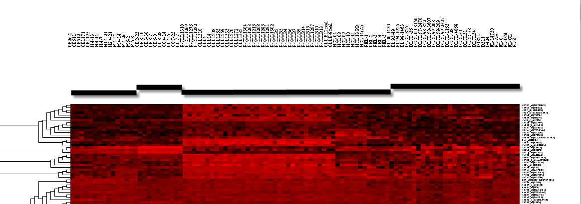
The results are placed in the Project Folders component and labeled "Hierarchical Clustering", and can be displayed in the Dendrogram component.

Displaying results in the Dendrogram component

Hierarchical clustering results are displayed in the Dendrogram component. The four horizontal bars shown in the diagram below were added just to show the boundaries of the four array sets used. (Note - you do not need to activate sets for clustering, unless you wish to use only a subset of all available arrays or markers).

Selecting a subtree

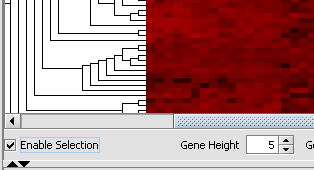
The Dendrogram component allows one to select and work with just a portion of the displayed tree. To activate this feature, check the Enable Selection checkbox at lower left in the Dendrogram component.

Now when the cursor is moved over the displayed tree, a blue rectangle will indicate which portion of the tree is currently sub-selected.

Clicking on the selected area will cause only this area to be displayed.

Working with a subtree in the Dendrogram

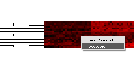
Right-clicking on the displayed sub-tree will show a menu with two entries:

• Image Snapshot - place a static snapshot of the tree as currently displayed into Project Folders component.

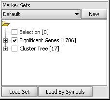
• Add to Set - add the markers represented in the currently displayed tree to a new set in the Markers component called "Cluster Tree".

The following figure shows the the new set of markers after it has been added to the Markers component.