geWorkbench

Outline

In this tutorial, you will:

• Discuss the background for using Student's t-Test to evaluate data.
• Load a geWorkbench matrix format microarray dataset.
• Select classes of arrays to compare.
• Apply a t-Test.
• Visualize the results in the Color Mosaic and Volcano Plot components.
• Note the creation of resulting marker lists and visualization objects.
• Apply a multi t-test.

Overview

A t-Test analysis can be used to identify markers with statistically significant differential expression between two sets of microarrays. The t-test determines, for each marker, if there is a significant difference between the two groups (e.g. case and control). To perform this analysis, you must classify the sets, set the analysis parameters and view the results in the visualization components. The t-test implementation in geWorkbench offers several options for multiple testing correction and evaluation of the test statistic. A detailed description of the t-Test parameters is also available in online help.

Preparation

Obtain the file "BCell-100.exp", which is contained in the data/public_data directory of the geWorkbench distribution, or can be directly downloaded from the tutorial data download area.

For tips on loading data files, see Local Data Files and Projects.

t-Test Parameters

P-value

The p-value can be estimated from 1. the t-statistic (the default) or 2. by permutation.

Alpha corrections

For multiple testing (alpha) correction, the following options are offered:

1. no correction
2. Standard Bonferonni Correction
3. Adjusted (step down) Bonferonni Correction.
4. Additional methods are available if the p-value is being estimated by permuation:
   1. minP
   2. maxT

Degrees of Freedom

Group variances can be declared as: 1. unequal (Welch approximation) (the default) 2. Equal.

Classification

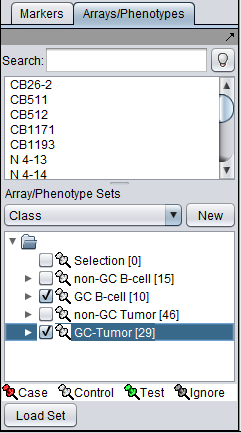
The desired sets of arrays should be activated in the Arrays/Phenotypes component. This is done by checking the boxes by the desired Sets.

The t-test requires two groups of microarrays to compare. geWorkbench distinguishes the two groups by one being labeled as "Case". By default, all others are considered as control. Note that in the Arrays/Phenotypes component, more than one set of arrays can be marked "Case". All remaining (activated) arrays will then be in the "Control" group.

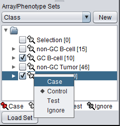
The classification can be made directly by left-clicking on the "thumb-tack" icon adjacent to an array set name.

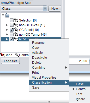
The array classification can also be set by right-clicking on the desired array set and selecting "Classification":

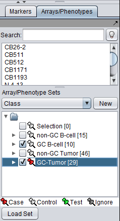
Using either method, the desired array set can be set to be classified as "Case":

The thumbtack image next to activated Array Sets is colored red.

Set Analysis Parameters

• From the Analysis Panel, select T-Test Analysis.
• Various parameters can be adjusted as desired. Here we will use the Standard Bonferonni method, which is the strictest.

• Alpha-corrections tab: Standard Bonferonni.

• P-Value Parameters tab: p-values based on t-distribution. Note that the default alpha (critical p-value) is set to 0.01.

• Degree of Freedom tab: Welch approximation - unequal group variances.

After all the parameters have been set, click Analyze. The results will be returned in three locations: The Project Folder, the Markers component, and the Visualization area.

t-Test Results

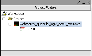
The result is placed into the Projects Folder as a child of the microarray dataset that was analyzed.

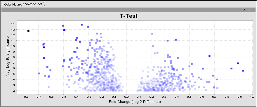
The results are displayed by default using the Volcano Plot visualizer.

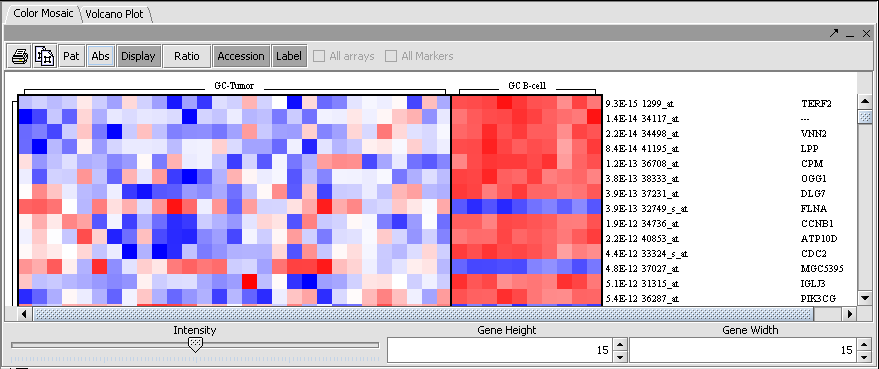
The adjacent tab provides a Color Mosaic showing all of the arrays and the p-value calculated for each marker. It also can display annotation for each marker.

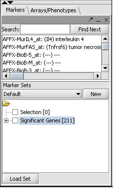
The set of markers which met the minimum signifcance criterion are placed into a new Marker Set labeled "Significant Genes" in the Markers component. The number of markers is shown also.

References

t-test [1]