Difference between revisions of "Basics"
(→Data representation) |
|||
| (46 intermediate revisions by 3 users not shown) | |||
| Line 1: | Line 1: | ||
| + | {{TutorialsTopNav}} | ||
| − | |||
| − | + | __TOC__ | |
| + | ==Introduction to geWorkbench== | ||
| + | geWorkbench (genomics Workbench) is a Java-based open-source platform for integrated genomics. Using a component architecture it allows individually developed plug-ins to be configured into complex bioinformatic applications. At present there are more than 70 available plug-ins supporting the visualization and analysis of gene expression and sequence data. Example use cases include: | ||
| − | + | * loading data from local or remote data sources. | |
| + | * visualizing gene expression, molecular interaction networks, protein sequence and protein structure data in a variety of ways. | ||
| + | * providing access to client- and server-side computational analysis tools such as t-test analysis, hierarchical clustering, self organizing maps, regulatory neworks reconstruction, BLAST searches, pattern/motif discovery, etc. | ||
| + | * validating computational hypothesis through the integration of gene and pathway annotation information from curated sources as well as through Gene Ontology enrichment analysis. | ||
| − | |||
| − | |||
| − | |||
| − | |||
| − | |||
| − | |||
| − | |||
| − | == | + | ==Layout of the Graphical User Interface== |
| − | |||
| − | |||
| − | |||
| − | |||
| − | |||
| − | |||
| − | |||
| − | |||
| − | |||
| − | |||
| − | |||
| + | The graphical user interface for geWorkbench is divided into three major sections, for | ||
| + | # (1) Data management - [[Workspace]] (upper left) | ||
| + | # (2) Visualization tools (right) | ||
| + | # (3) Marker and Array/Phenotype set selection and management (lower left) | ||
| − | |||
| + | [[Image:GeWorkbench_full_GUI_color_mosaic.png|{{ImageMaxWidth}}]] | ||
| − | + | Commands for analysis, filtering and normalization are now available in a menu activated by right-clicking on any loaded data node. They can also be found in the top level menu-bar under "Commands". They will act on the currently selected data node. | |
| + | [[Image:Basics_Analysis_t-test.png]] | ||
| + | ==Window Decorations== | ||
| − | + | Each component within an area is resizable and detachable. | |
| + | '''Undock''' | ||
| + | * The Undock button is an arrow pointing up and to the right. | ||
| + | * Clicking on the Undock icon detaches the component. It can then be expanded and positioned at will on the screen. | ||
| + | * In the detached component, the Dock icon is a left-downward arrow. Clicking on the Dock icon reattaches the panel within its GUI area. | ||
| + | '''Sizing Arrows''' | ||
| + | * To resize an area discretely (maximize/minimize), click on the triangular-shaped wedges located within the separators between panels. Maximizing a panel fills the entire window vertically or horizontally, and minimizes the adjacent panel. | ||
| + | [[Image:Window_decorations.png]] | ||
| − | |||
| − | + | '''Sizing Handle''' | |
| + | * Any separator between two panes that has a sizing handle can be moved by right- or left-clicking anywhere on the separator and dragging the edge. | ||
| − | |||
| − | + | [[Image:Window_separator_handle.png]] | |
| − | + | ==Command Popup== | |
| + | Hitting F12 on the keyboard will pop-up a shortcut menu to the geWorkbench commands available for the current dataset. | ||
| − | + | [[Image:F12-Popup.png]] | |
| − | |||
| − | |||
| − | |||
| − | |||
| − | |||
| − | |||
| + | ==Data management area== | ||
| + | The [[Workspace]] is a top-level geWorkbench component that holds data, analysis results, images, sequences, networks and other types of input and output. A [[Workspace]] and all the data within it can be saved and later reloaded. Only one [[Workspace]] at a time can be open. These operations will be described in detail in further sections of the tutorials. | ||
| + | |||
The GUI provides a menu bar at top with a standard choice of commands. Many commands that are available in the menu bar are also available by right-clicking on data objects. | The GUI provides a menu bar at top with a standard choice of commands. Many commands that are available in the menu bar are also available by right-clicking on data objects. | ||
| − | + | ==Set selection and management== | |
| − | |||
| − | |||
| − | |||
| − | |||
| − | |||
| − | |||
| − | |||
| − | |||
| − | |||
| − | + | A key feature of geWorkbench is the ability to work with defined sets of markers or arrays. This allows subsets of data to be analyzed, and allows for passing of selected subsets of data between different components. For example, the t-test produces a list of markers showing a significant difference in expression between two states, and this list can then be used to retrieve relevant sequences or annotations. | |
| − | + | ==Visualization and Analysis tools== | |
| + | geWorkbench works such that only the visualization and analysis components relevant to the type of dataset currently selected in the [[Workspace]] area (1) are displayed in the Visualization Area (2) or in the command menus. Thus choosing a microarray dataset will result in a different set of visualizers being displayed as compared with those seen when a nucleotide sequence file is selected. When a new data file is loaded, or an analysis produces a new data set, not only is it added to the [[Workspace]] (1), but an appropriate viewer in the Visualization area (2) is automatically selected. | ||
| − | + | ==Component Interoperability== | |
| + | The features described above underly the most important design goal of geWorkbench, which is to allow the different components to interoperate easily. The user is freed of the need to write programs to convert data from one format to another for different programs. Both the [[Workspace]] (1) and the Set Selection component(3) can hold shared data. Typically each run of an analysis places either a new dataset into the [[Workspace]], or a new set of markers or arrays into the Set Selection component. These are then available to any other appropriate component for reuse. | ||
| − | |||
| + | ==Data representation== | ||
| − | + | geWorkbench works on a single dataset at one time, as selected in the [[Workspace]]. For working with data from multiple microarrays simultaneously, for example for statistical analysis or clustering, all of the data must be represented as a single two-dimensional array of experiments and markers. Such a representation can be created externally, for example in Excel, or geWorkbench can read in expression results from single arrays and merge them into a combined dataset. The merging process is described in detail in [[Local_Data_Files#Merging_Microarray_Files|Local Data Files]] and also in [[Menu_Bar#Merge_Datasets|Menu Bar]]. | |
| + | An option at the time of file read-in allows multiple files to be opened and merged simultaneously, either from disk or from remote data sources such as caArray. Alternatively, single datasets that have already been read-in can also be merged at a later time. Either route creates a single data object in the [[Workspace]] representing all of the arrays. This object can be viewed, for example, using the color mosaic component. The merged representation can be saved to the geWorkbench *.exp file type. | ||
| − | + | The results of any data analysis are stored in the [[Workspace]] as a child of the dataset from which they were created. | |
| − | + | ==Limitations== | |
| − | + | As currently implemented, operations such as filtering and normalization directly alter the loaded dataset. However, the original data file is not changed. | |
Latest revision as of 14:42, 22 April 2014
Contents
Introduction to geWorkbench
geWorkbench (genomics Workbench) is a Java-based open-source platform for integrated genomics. Using a component architecture it allows individually developed plug-ins to be configured into complex bioinformatic applications. At present there are more than 70 available plug-ins supporting the visualization and analysis of gene expression and sequence data. Example use cases include:
- loading data from local or remote data sources.
- visualizing gene expression, molecular interaction networks, protein sequence and protein structure data in a variety of ways.
- providing access to client- and server-side computational analysis tools such as t-test analysis, hierarchical clustering, self organizing maps, regulatory neworks reconstruction, BLAST searches, pattern/motif discovery, etc.
- validating computational hypothesis through the integration of gene and pathway annotation information from curated sources as well as through Gene Ontology enrichment analysis.
Layout of the Graphical User Interface
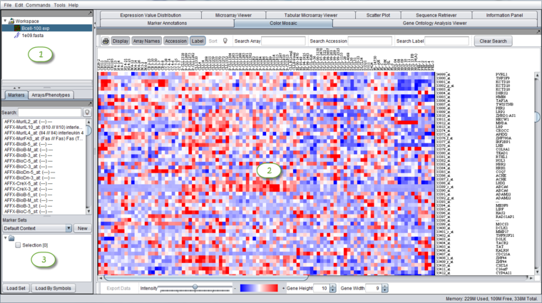
The graphical user interface for geWorkbench is divided into three major sections, for
- (1) Data management - Workspace (upper left)
- (2) Visualization tools (right)
- (3) Marker and Array/Phenotype set selection and management (lower left)
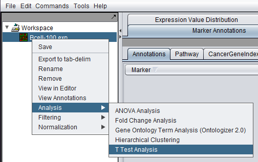
Commands for analysis, filtering and normalization are now available in a menu activated by right-clicking on any loaded data node. They can also be found in the top level menu-bar under "Commands". They will act on the currently selected data node.
Window Decorations
Each component within an area is resizable and detachable.
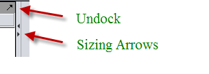
Undock
- The Undock button is an arrow pointing up and to the right.
- Clicking on the Undock icon detaches the component. It can then be expanded and positioned at will on the screen.
- In the detached component, the Dock icon is a left-downward arrow. Clicking on the Dock icon reattaches the panel within its GUI area.
Sizing Arrows
- To resize an area discretely (maximize/minimize), click on the triangular-shaped wedges located within the separators between panels. Maximizing a panel fills the entire window vertically or horizontally, and minimizes the adjacent panel.
Sizing Handle
- Any separator between two panes that has a sizing handle can be moved by right- or left-clicking anywhere on the separator and dragging the edge.
Command Popup
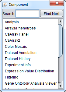
Hitting F12 on the keyboard will pop-up a shortcut menu to the geWorkbench commands available for the current dataset.
Data management area
The Workspace is a top-level geWorkbench component that holds data, analysis results, images, sequences, networks and other types of input and output. A Workspace and all the data within it can be saved and later reloaded. Only one Workspace at a time can be open. These operations will be described in detail in further sections of the tutorials.
The GUI provides a menu bar at top with a standard choice of commands. Many commands that are available in the menu bar are also available by right-clicking on data objects.
Set selection and management
A key feature of geWorkbench is the ability to work with defined sets of markers or arrays. This allows subsets of data to be analyzed, and allows for passing of selected subsets of data between different components. For example, the t-test produces a list of markers showing a significant difference in expression between two states, and this list can then be used to retrieve relevant sequences or annotations.
Visualization and Analysis tools
geWorkbench works such that only the visualization and analysis components relevant to the type of dataset currently selected in the Workspace area (1) are displayed in the Visualization Area (2) or in the command menus. Thus choosing a microarray dataset will result in a different set of visualizers being displayed as compared with those seen when a nucleotide sequence file is selected. When a new data file is loaded, or an analysis produces a new data set, not only is it added to the Workspace (1), but an appropriate viewer in the Visualization area (2) is automatically selected.
Component Interoperability
The features described above underly the most important design goal of geWorkbench, which is to allow the different components to interoperate easily. The user is freed of the need to write programs to convert data from one format to another for different programs. Both the Workspace (1) and the Set Selection component(3) can hold shared data. Typically each run of an analysis places either a new dataset into the Workspace, or a new set of markers or arrays into the Set Selection component. These are then available to any other appropriate component for reuse.
Data representation
geWorkbench works on a single dataset at one time, as selected in the Workspace. For working with data from multiple microarrays simultaneously, for example for statistical analysis or clustering, all of the data must be represented as a single two-dimensional array of experiments and markers. Such a representation can be created externally, for example in Excel, or geWorkbench can read in expression results from single arrays and merge them into a combined dataset. The merging process is described in detail in Local Data Files and also in Menu Bar.
An option at the time of file read-in allows multiple files to be opened and merged simultaneously, either from disk or from remote data sources such as caArray. Alternatively, single datasets that have already been read-in can also be merged at a later time. Either route creates a single data object in the Workspace representing all of the arrays. This object can be viewed, for example, using the color mosaic component. The merged representation can be saved to the geWorkbench *.exp file type.
The results of any data analysis are stored in the Workspace as a child of the dataset from which they were created.
Limitations
As currently implemented, operations such as filtering and normalization directly alter the loaded dataset. However, the original data file is not changed.
