Difference between revisions of "SOM"
| Line 53: | Line 53: | ||
[[Image:T_HierarchicalClustering_BC44Markers.png]] | [[Image:T_HierarchicalClustering_BC44Markers.png]] | ||
| + | |||
| + | |||
| + | This will result in two sets of markers having been added to the Markers component, as shown below: | ||
| + | |||
| + | [[Image:T_Markers_ClusterTree12and44.png]] | ||
Revision as of 20:33, 24 April 2006
Preparation: An example of filtering and normalization
The file "webmatrix.exp" contains results from 100 Affymetrix HG-U95Av2 chips containing B-cell samples from numerous different disease states (phenotypes). 12600 markers are represented. To prepare this dataset for clustering we will normalize and filter the data. The steps shown below are just an example of how filtering and normalization can be used, and each dataset should be handled according to the type of analysis being undertaken and its goals.
The dataset was created by the following steps:
- Normalization: Quantile normalization.
- Normalization: Log2 transformation.
- Filtering: Deviation filter with Deviation bound of 1.
- Filtering: Missing values filter with maximum number of missing arrays of 0.
The results of performing these steps are also available as the file "webmatrix_quantile_log2_dev1_mv0.exp" in the tutorial data section (coming soon).
Example
- In the Arrays/Phenotypes component, select the set of arrays labeled "ultrashort designation".
- Activate two classes of arrays to compare, the GC B-cell and non-GC B-cell, by checking the boxes before the names.
- Go to the Analysis component, and select Hierarchical Clustering.
- At the bottom of the Analysis component, uncheck the box that says "All Arrays". This will allow the clustering to be done only on those arrays which were activated in the Arrays/Phenotypes component.
- In Hierarchical Clustering, set the parameters to:
- Clustering Method: Total Linkage
- Clustering Dimension: Both
- Clustering Metric: Euclidean
- Click Analyze.
The results will be displayed in the Dendrogram component.
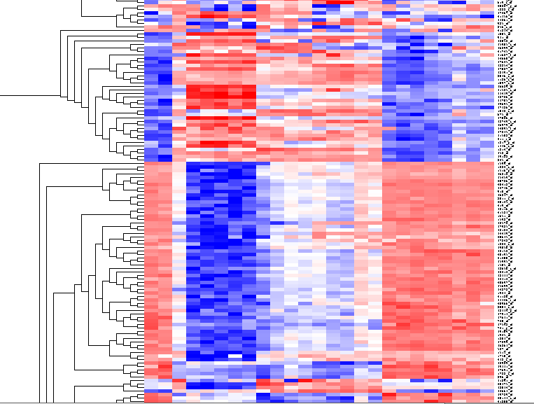
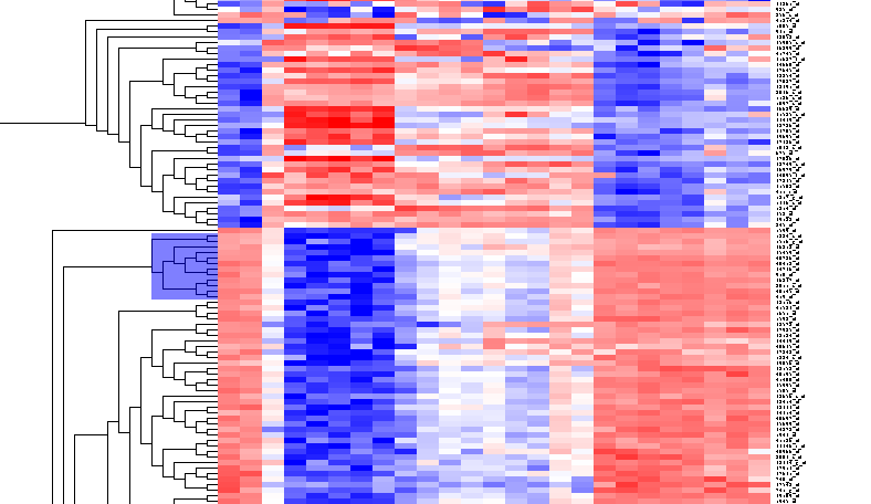
By scrolling down a bit, one finds a large interesting area, showing clear differences between groups of arrays. We will select two clearly differentiated clusters. Check the Enable Zoom checkbox. Then highlight the first cluster of 12 markers as shown here:
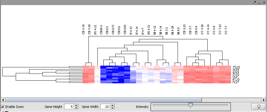
Then left-click to select this subset of the dendrogram. It will be displayed alone.
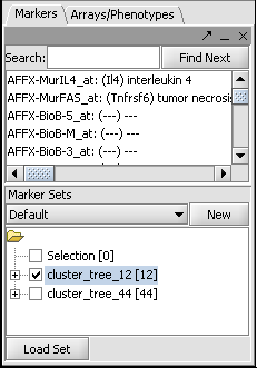
Now right-click and select "Add to Set". In the Markers component, the select genes are added as Cluster Tree [12], where 12 is the number of markers selected.
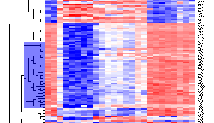
Repeat for the similar region just below, which contains another 44 markers.
This will result in two sets of markers having been added to the Markers component, as shown below:
