Revision as of 20:22, 27 February 2006 (view source) Smith (talk | contribs) ← Older edit		Latest revision as of 17:07, 10 January 2014 (view source) Smith (talk | contribs) (→‎Overview)
(168 intermediate revisions by 4 users not shown)
Line 1:		Line 1:
	{{TutorialsTopNav}}		{{TutorialsTopNav}}
−	==Outline==	+	==Overview==
−	In this tutorial, you will learn how to:
−	*Create a new Project.
−	*Load microarray data.
−	*Merge data from several loaded microarray experiments.
−	*Rename a project and/or project node.
−	*Remove a project and/or project node.
−	*Save project files that you have created.
−	*Load, add, and/or modify remote data.
		+	The Workspace is located in the upper-left-hand corner of the application. It is used to contain open data files and store analysis results during a geWorkbench session. When geWorkbench is launched, an empty Workspace folder is displayed.
−	===Supported data formats===	+	[[Image:Workspace.png]]
−	*Microarray
−	**Affymetrix MAS5/GCOS Files.'''''This one will be used for the tutorial.'''''  ''brief explanation of file type needed''
−	**Affymetrix File Matrix - this is the native file type created by geWorkbench.
−	**RMA Express File - RMA Express is a sophisticated tool for combining data from multiple Affymetrix chips.
−	**Affy Excel or txt data file.
−	**Normalized no-confidence expression matrix. A variant of the geWorkbench file matrix format that omits the confidence value columns (P-value or Present/Absent calls).
−	**Genepix Files - An analysis program for two color arrays.
−	*Other
−	**FASTA Files. DNA or protein sequence files in FASTA format.
−	**Pattern Files.
−	**Genotypic data Files.
		+	The workspace as a whole, with all its projects and data nodes, can be saved and restored.  However, only one workspace can be open at one time.  Creating a new workspace or loading a saved workspace will overwrite the current workspace.
−	===Workspaces and Projects===
−	'''1.'''To create a New Project, right-click on Workspace in the Project Folders area at upper left.
−	[[Image:Loadingdata1.jpg]]
		+	* To view the next level down in the hierarchy, click on the “+” icon to expand the branch.
−	'''2.''' Left-click on Project.	+	* To collapse a branch, click on the “-” icon.
−	[[Image:(T)Loadingdata.png]]
		+	The Workspace may contain several heterologous datasets. These datasets can include input (source) data and derived data (results) associated with an experiment as well as image files. Source data can be loaded from the user’s local storage or from remote servers.  Loading datasets into the geWorkbench Workspace does not change their physical storage locations.
−	'''3.''' a new Project folder will be created. right-click on it, then left-click on open files.	+	'''Note''' - The top menu-bar items [[Menu_Bar#File|File]] and [[Menu_Bar#Edit|Edit]] also apply to items in the Workspace. They offer many of the same options shown below, except e.g. Microarray merging is only available from the top level [[Menu_Bar#File|File]] menu.
−	[[Image:(T)Loadingdata1.png]]	+	==Workspace Menu Options==
		+	Right-clicking on the Workspace node gives a menu with the following options
−	'''4.''' Find the type of file that you want to work with. '''''In this case it will be Affymetrix MAS5/GCOS Files.'''''
−	'''5.''' Find the file that you want to work with and select.	+	[[Image:Workspace_right_click_menu.png]]
−	'''6.''' Make sure '''Local''' radio button is selected.
−	'''7.''' Click on the '''Open''' button.	+	===Open Files===
		+	* Loading data from local files is covered in the chapter [[Local_Data_Files | Local Data Files]]
		+	* Retrieving data from remote sources (caArray) is covered in [[Remote_Data_Sources | Remote Data Sources]]
−	[[Image:(T)MFileScreen.png]]
−	Your File is now loaded:	+	===Open PDB File from RCSB Protein Data Bank===
		+	If '''Open PDB File from RCSB Protein Data Bank''' is chosen, a dialog box appears.
−	[[Image: (T)MLoadingData.png]]
		+	[[Image:Project_Folders_Project_Open_RCSB_PDB.png]]
−	'''<u>You Can Merge Data From Several Loaded Microarray Experiments Into One Project Folder</u>'''
−	Different Microarray files can be merged so that they can be viewed and analyzed together. As long as files are of the same type you can merge them into one project node.	+	Type in the name of a PDB structure entry and it will be retrieved from the RCSB Protein Data Bank and loaded into geWorkbench.
−	You can do this during the original loading process, or after you have already loaded a file.
		+	==Workspace Data Node Menu Options==
		+	Right-clicking on a data node will produce a popup menu with the following options:
−	'''''<u>To Merge Data From The Original Loading Process</u>'''''
−	'''1.''' Right mouse click on the Project folder.	+	[[Image:Workspace_data_node_right_click.png]]
−	'''2.''' Select the files that you want to Merge.
−	'''3.''' Select the Merge Files box.	+	===Save===
−	'''4.''' Left mouse click on the '''Open''' button.	+	Save the currently selected data node.  This is implemented for at least the below data types. If saving of a particular type has not been implemented, the "Save" option will be disabled (grayed-out).
−	[[Image:(T)Merge.png]]	+	* '''Microarray gene expression''' -  data is saved using the geWorkbench ".exp" format, regardless of the original format. This allows saving e.g. a merged dataset, and/or any array and marker sets that may have been created.
		+	* '''FASTA''' - saved in FASTA format (.fasta).
		+	* '''PDB''' - saved in PDB format (.pdb).
		+	* '''Network''' - saved using the Adjacency Matrix "ADJ" format (.adj).
		+	* '''t-test result''' - saved as comma separated value (.csv) file.
		+	* '''Image''' - saved as PNG file (.png).
−	Your File Nodes will now be Merged into one Project folder.	+	For each file type, a file browser with a filter for the target file type extension (e.g. .fasta) will be opened.
−	[[Image:(T)MLoadingData1.png]]	+	===Export to tab-delim===
		+	This option will only appear for microarray gene expression datasets.  It allows the microarray dataset to be exported in a spreadsheet format, as a tab-delimited text file.  The first row contains array names and the first column contains the marker names.
−	'''''<u>To Merge Data From Experiments Already Loaded</u>'''''	+	This export format does not preserve array or marker sets that may have been defined in geWorkbench for the dataset.  However, it can be used to save a copy of e.g. merged, filtered, and/or normalized data in a format easily used by other programs.
−	'''1.''' Select the Project Nodes that you want to Merge.	+	When exporting, the file save dialog will display the name of the dataset, minus any recognized file-type suffixes that may be present (e.g. .soft).
−	'''2.''' Left click on file, choose Merge Datasets.	+	===Rename===
−	[[Image:(T)MFileScreen1.png]]	+	A dialog box will appear in which a new name can be entered.
−	'''<u>You Can Rename a Project and/or a Project Node</u>'''	+	[[Image:Workspace_Rename_Node.png]]
		+	===Remove===
−	'''<u>''Renaming A Project''</u>'''	+	The selected data nodes and any child data nodes will be removed.  Multiple selections can be made.
−	'''1.''' Right mouse click on Project folder.	+	==Data Node Hover-text Information==
−	'''2.''' Select Rename.	+	For microarray datasets, adjacency matrices (network nodes), sequence and pattern nodes, moving the mouse cursor over the data nodes will display additional details about a dataset.
−	[[Image:(T)MReNameProject.png]]	+	Microarray datasets: hover text displays number of markers and arrays.
−	'''3.''' In Pop-up Screen Rename your Project.
−	'''4.''' Click on the '''Okay''' button	+	[[Image:Dataset_hover_microarray.png]]
−	'''<u>''Renaming a Project Node''</u>'''	+	Adjacency Matrix: hover text displays number of nodes and edges in the network.
−	'''1.''' Right mouse click on Project Node.
−	'''2.''' Select Rename.	+	[[Image:Workspace_Dataset_hover_network.png]]
−	[[Image:(T)MReNameProjectNode.png]]
−	'''3.''' In Pop-up Screen Rename your Project Node.	+	Sequence node:
−	'''4.''' Click on the '''Okay''' button.
		+	[[Image:Workspace_hover_sequences.png]]
		+	Pattern node:
−	'''<u>You Can Remove a Project and/or a Project Node</u>'''
		+	[[Image:Workspace_Pattern_Hover.png]]
−	'''<u>''Removing A Project''</u>'''	+	==Workspaces==
−	'''1.''' Right mouse click on Project folder.	+	===Saving the Workspace===
−	'''2.''' Select Remove.	+	Saving the workspace saves all its data to a file on disk. The workspace can later be reloaded to resume work.
−	'''3.''' You will no longer see the Project folder.	+	====Special considerations on saving and restoring workspaces====
		+	* '''Versions''' - Workspaces in general may not be compatible across different versions of geWorkbench.
		+	* '''Loaded components''' - The configuration in the [[Component_Configuration_Manager| CCM]] of which components are loaded and which are not is not saved when the workspace is saved; it is maintained separately.
		+	* '''Changes to loaded components''' - If a workspace is saved, and then changes are made to which components are loaded in the [[Component_Configuration_Manager| CCM]], then in rare cases problems may occur when one attempts to reload the saved workspace.
−	'''<u>''Removing a Project Node''</u>'''	+	[[Image:File_Save_Workspace.png]]
−	'''1.''' Right mouse click on Project Node.	+	===Opening a Saved Workspace===
−	'''2.''' Select Remove Project.	+	File->Open-Workspace.
−	'''3.''' You will no longer see the Project Node.	+	Only one workspace at a time can be loaded in geWorkbench. Opening a saved workspace will destroy the existing workspace.  For this reason, if you opt to open a workspace, you will be prompted as to whether to save the existing workspace first.
−	'''<u>''Saving a File 'Node'</u>'''	+	[[Image:File_Open_Workspace.png]]
−	'''1.''' Right mouse click on File(s) 'Node(s)' that you want to save.
−	'''2.''' Click on the Save.'''	+	A dialog box will appear in which the location and file name to which to save the workspace can be chosen.
−	[[Image:(T)MSavingAFile.png]]	+	[[Image:File_Save_Workspace_Dialog.png]]
−	The Save Screen will come up.	+	===Creating a New Workspace===
−	[[Image:(T)MSavingAFile1.png]]	+	Only one workspace at a time can be loaded in geWorkbench.  Creating a new workspace will destroy the existing workspace.  For this reason, if you opt to create a new workspace, you will be prompted as to whether to save the existing workspace first.
−	'''3.''' Choose a location.	+	A new workspace can only be created from the top level menu bar.
−	'''4.''' Name your File(s) 'Node(s)'
−	'''5.''' Click on the '''Save''' button	+	[[Image:File_New_Workspace.png]]
−	'''<u>Load, Add, and/or Modify Remote Data</u>'''	+	Select '''File->New->Workspace'''.
−
−	There will be times that you may need data from a Remote Location, with this program you are able to load, add, and/or modify that data.
−
−	When the File Screen comes up click on the Remote Radial button and you will see this screen.
−	The Open File Dialog Window is updated so that you can work with your Remote Sources.
−
−	[[Image:(T)MEditRemoteData.png]]
−
−	The four buttons on the bottom of this screen are what you will be working with
−
−	'''''Basic Usage'''''
−
−	'''caArray''' button - Gives you a listing of your Remote Resources.
−
−	'''Go''' button - Accesses the Remote Source that you selected.
−
−	'''Add A New Resource''' button - Opens the Data Source Definition Page used to add Remote Data.
−
−	'''Edit''' button - Edits Remote Source Parameters.
−
−
−	'''''To Add A Remote Source'''''
−
−	'''1.''' Click on the '''Add A New Resource''' button.
−
−	[[Image:(T)MRemoteData2.png]]
−	This is the Data Source Definition Page
−
−	'''2.''' Fill in the Data Source definition page. URL and Short Name are required fields.
−
−	'''3.''' Click on the OK button.
−
−	The configuration is set up to automatically reflect your additional Data Source.
−
−
−	'''''To Modify A Remote Source'''''
−
−	'''1.''' Select the File that you want to modify.
−
−	[[Image:(T)MRemoteData1.1.png]]
−
−	'''2.''' Click on the '''Edit''' button.
−
−
−	[[Image:(T)MRemoteData3.png]]
−
−	'''3.''' Make the changes that you need.
−
−	'''4.''' Click on the '''OK''' button
−
−	End Mary::::::::::::::
−
−
−
−	===Loading Data===
−
−	When first started, geWorkbench appears so:
−
−	[[Image:T_StartupState.png]]
−
−
−	Right-click on the '''Workspace''' entry in the '''Project Folders''' window at upper left to create a new project.
−
−	[[Image:T_NewProject.png]]
−
−
−
−	Next, right-click on the new project entry and select '''Open Files'''.
−
−	[[Image:T_OpenFiles.png]]
−
−
−
−	Here we will select 10 MAS5 format text files from the directory geworkbench\data\training\cardiogenomics.med.harvard.edu, which is included in the geWorkbench download:
−
−	[[Image:T_SelectMAS5.png]]
−
−
−
−	The chip type HG_U95Av2 is recognized...
−
−	[[Image:T_Chip_type_message.png]]
−
−
−
−	The read-in data is displayed in the '''Microarray Panel'''.  Note we have increased the instensity slider to maximum here.
−
−	[[Image:T_MAS5_display.png]]
−
−
−
−	We can now assign phenotypes to each chip.  We will place the phenotypes in the default group, however you can create new phenotype groups by pushing the '''New''' button on the '''Phenotype Panel''' at lower left.
−
−	Here we select and label arrays in the '''Phenotype Panel''' which contain samples from the congestive cardiomyopathy disease state...
−
−	[[Image:T_PanelLabelCardio.png]]
−
−
−
−	Next, we can similarly label the remaining arrays as "Normal".  We have also checked boxes to indicate that these groups of arrays are "Active".  Various analysis and visualization components can be set to only use/display activated arrays or markers.
−
−	[[Image:T_PhenotypesPriorToCase.png]]
−
−
−
−	For statistical tests such as the t-test the Case and Control groups can be specified.  This is done by left-clicking on the thumb-tack icon in front of the phenotype name.  Here we are specifying the disease arrays as the "Case".  The remaining "Normal" arrays are by default labeled control.
−	[[Image:T_PhenotypeSettingCase.png]]
−
−
−
−	A red thumbtack indicates the arrays have been specified as "Case".
−
−	[[Image:T_PhenotypeCaseSet.png]]
−
−
−
−	We can also rename the merged dataset by clicking on its entry in the '''Project Panel'''.
−
−	[[Image:T_RenameDataset.png]]
−
−
−
−	Here we will call it CCMP.
−
−	[[Image:T_RenamingDataset.png]]
−
−
−
−	With the datasets merged, classified and named, we can save the dataset for future use. We will call it "cardiomyopathy.exp" (.exp is the default extension for the geWorkbench matrix file type).
−
−	[[Image:T_SaveProject.png]]
−
−
−
−	The default display of microarray data is an absolute display.  We can change it to a relative display by selecting Tools:Preferences from the top menubar.  We have removed the dataset so that we can read it back in using the new preferences.
−
−	[[Image:T_ChangePrefs.png]]
−
−
−
−	Here we select the '''relative''' display type.
−
−	[[Image:T_ChangePrefsToRelative.png]]
−
−
−
−	Returning to the Open File dialog as we before by right-clicking on the project entry, we will select the "cardiomyopathy.exp" file we previously saved...
−
−	[[Image:T_OpenCardio.png]]
−
−
−
−	Resulting in the following colorful display of the array data for the first array....
−
−	[[Image:T_RelativeDisplay.png]]
−
−
−
−
−
−	[[Image:(T)MarGettingStarted.png]]

---

Latest revision as of 17:07, 10 January 2014

Home | Quick Start | Basics | Menu Bar | Preferences | Component Configuration Manager | Workspace | Information Panel | Local Data Files | File Formats | caArray | Array Sets | Marker Sets | Microarray Dataset Viewers | Filtering | Normalization | Tutorial Data | geWorkbench-web Tutorials

Analysis Framework | ANOVA | ARACNe | BLAST | Cellular Networks KnowledgeBase | CeRNA/Hermes Query | Classification (KNN, WV) | Color Mosaic | Consensus Clustering | Cytoscape | Cupid | DeMAND | Expression Value Distribution | Fold-Change | Gene Ontology Term Analysis | Gene Ontology Viewer | GenomeSpace | genSpace | Grid Services | GSEA | Hierarchical Clustering | IDEA | Jmol | K-Means Clustering | LINCS Query | Marker Annotations | MarkUs | Master Regulator Analysis | (MRA-FET Method) | (MRA-MARINa Method) | MatrixREDUCE | MINDy | Pattern Discovery | PCA | Promoter Analysis | Pudge | SAM | Sequence Retriever | SkyBase | SkyLine | SOM | SVM | T-Test | Viper Analysis | Volcano Plot

Overview

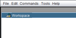
The Workspace is located in the upper-left-hand corner of the application. It is used to contain open data files and store analysis results during a geWorkbench session. When geWorkbench is launched, an empty Workspace folder is displayed.

The workspace as a whole, with all its projects and data nodes, can be saved and restored. However, only one workspace can be open at one time. Creating a new workspace or loading a saved workspace will overwrite the current workspace.

• To view the next level down in the hierarchy, click on the “+” icon to expand the branch.

• To collapse a branch, click on the “-” icon.

The Workspace may contain several heterologous datasets. These datasets can include input (source) data and derived data (results) associated with an experiment as well as image files. Source data can be loaded from the user’s local storage or from remote servers. Loading datasets into the geWorkbench Workspace does not change their physical storage locations.

Note - The top menu-bar items File and Edit also apply to items in the Workspace. They offer many of the same options shown below, except e.g. Microarray merging is only available from the top level File menu.

Workspace Menu Options

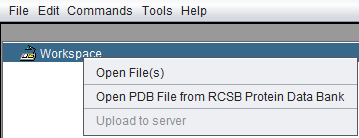
Right-clicking on the Workspace node gives a menu with the following options

Open Files

• Loading data from local files is covered in the chapter Local Data Files
• Retrieving data from remote sources (caArray) is covered in Remote Data Sources

Open PDB File from RCSB Protein Data Bank

If Open PDB File from RCSB Protein Data Bank is chosen, a dialog box appears.

Type in the name of a PDB structure entry and it will be retrieved from the RCSB Protein Data Bank and loaded into geWorkbench.

Workspace Data Node Menu Options

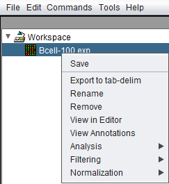
Right-clicking on a data node will produce a popup menu with the following options:

Save

Save the currently selected data node. This is implemented for at least the below data types. If saving of a particular type has not been implemented, the "Save" option will be disabled (grayed-out).

• Microarray gene expression - data is saved using the geWorkbench ".exp" format, regardless of the original format. This allows saving e.g. a merged dataset, and/or any array and marker sets that may have been created.
• FASTA - saved in FASTA format (.fasta).
• PDB - saved in PDB format (.pdb).
• Network - saved using the Adjacency Matrix "ADJ" format (.adj).
• t-test result - saved as comma separated value (.csv) file.
• Image - saved as PNG file (.png).

For each file type, a file browser with a filter for the target file type extension (e.g. .fasta) will be opened.

Export to tab-delim

This option will only appear for microarray gene expression datasets. It allows the microarray dataset to be exported in a spreadsheet format, as a tab-delimited text file. The first row contains array names and the first column contains the marker names.

This export format does not preserve array or marker sets that may have been defined in geWorkbench for the dataset. However, it can be used to save a copy of e.g. merged, filtered, and/or normalized data in a format easily used by other programs.

When exporting, the file save dialog will display the name of the dataset, minus any recognized file-type suffixes that may be present (e.g. .soft).

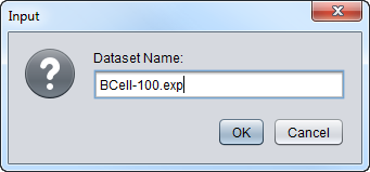
Rename

A dialog box will appear in which a new name can be entered.

Remove

The selected data nodes and any child data nodes will be removed. Multiple selections can be made.

Data Node Hover-text Information

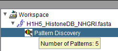
For microarray datasets, adjacency matrices (network nodes), sequence and pattern nodes, moving the mouse cursor over the data nodes will display additional details about a dataset.

Microarray datasets: hover text displays number of markers and arrays.

Adjacency Matrix: hover text displays number of nodes and edges in the network.

Sequence node:

Pattern node:

Workspaces

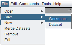
Saving the Workspace

Saving the workspace saves all its data to a file on disk. The workspace can later be reloaded to resume work.

Special considerations on saving and restoring workspaces

• Versions - Workspaces in general may not be compatible across different versions of geWorkbench.
• Loaded components - The configuration in the CCM of which components are loaded and which are not is not saved when the workspace is saved; it is maintained separately.
• Changes to loaded components - If a workspace is saved, and then changes are made to which components are loaded in the CCM, then in rare cases problems may occur when one attempts to reload the saved workspace.

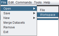
Opening a Saved Workspace

File->Open-Workspace.

Only one workspace at a time can be loaded in geWorkbench. Opening a saved workspace will destroy the existing workspace. For this reason, if you opt to open a workspace, you will be prompted as to whether to save the existing workspace first.

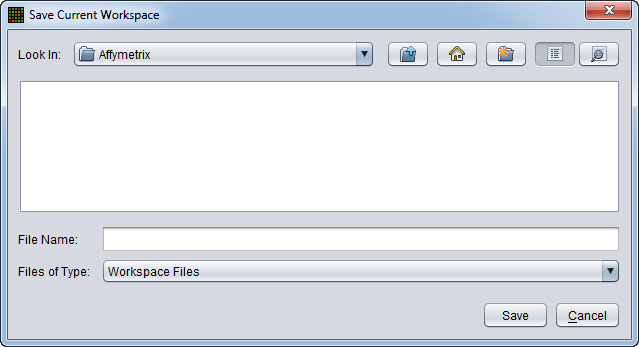
A dialog box will appear in which the location and file name to which to save the workspace can be chosen.

Creating a New Workspace

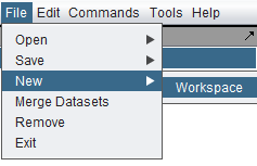
Only one workspace at a time can be loaded in geWorkbench. Creating a new workspace will destroy the existing workspace. For this reason, if you opt to create a new workspace, you will be prompted as to whether to save the existing workspace first.

A new workspace can only be created from the top level menu bar.

Select File->New->Workspace.