Difference between revisions of "Workspace"
| Line 1: | Line 1: | ||
| + | {{TutorialsTopNav}} | ||
| + | |||
| + | ==Outline== | ||
| + | In this tutorial, you will learn how to: | ||
| + | |||
| + | *Create a new Project. | ||
| + | *Load microarray data. | ||
| + | *Merge data from several loaded microarray experiments. | ||
| + | *Rename a project and/or project node. | ||
| + | *Remove a project and/or project node. | ||
| + | *Save project files that you have created. | ||
| + | *Load, add, and/or modify remote data. | ||
| + | |||
| + | |||
| + | |||
| + | ===Supported data formats=== | ||
| + | *Microarray | ||
| + | **Affymetrix MAS5/GCOS Files.'''''This one will be used for the tutorial.''''' ''brief explanation of file type needed'' | ||
| + | **Affymetrix File Matrix - this is the native file type created by geWorkbench. | ||
| + | **RMA Express File - RMA Express is a sophisticated tool for combining data from multiple Affymetrix chips. | ||
| + | **Affy Excel or txt data file. | ||
| + | **Normalized no-confidence expression matrix. A variant of the geWorkbench file matrix format that omits the confidence value columns (P-value or Present/Absent calls). | ||
| + | **Genepix Files - An analysis program for two color arrays. | ||
| + | *Other | ||
| + | **FASTA Files. DNA or protein sequence files in FASTA format. | ||
| + | **Pattern Files. | ||
| + | **Genotypic data Files. | ||
| + | |||
| + | |||
| + | |||
| + | ===Workspaces and Projects=== | ||
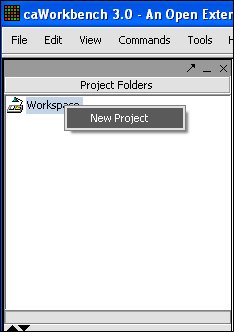
| + | '''1.'''To create a New Project, right-click on Workspace in the Project Folders area at upper left. | ||
| + | |||
| + | [[Image:Loadingdata1.jpg]] | ||
| + | |||
| + | |||
| + | '''2.''' Left-click on Project. | ||
| + | |||
| + | [[Image:(T)Loadingdata.png]] | ||
| + | |||
| + | |||
| + | '''3.''' a new Project folder will be created. right-click on it, then left-click on open files. | ||
| + | |||
| + | [[Image:(T)Loadingdata1.png]] | ||
| + | |||
| + | |||
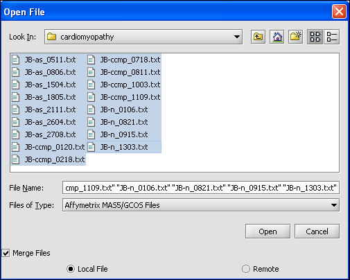
| + | '''4.''' Find the type of file that you want to work with. '''''In this case it will be Affymetrix MAS5/GCOS Files.''''' | ||
| + | |||
| + | '''5.''' Find the file that you want to work with and select. | ||
| + | |||
| + | '''6.''' Make sure '''Local''' radio button is selected. | ||
| + | |||
| + | '''7.''' Click on the '''Open''' button. | ||
| + | |||
| + | [[Image:(T)MFileScreen.png]] | ||
| + | |||
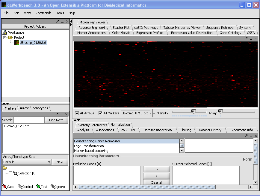
| + | Your File is now loaded: | ||
| + | |||
| + | [[Image: (T)MLoadingData.png]] | ||
| + | |||
| + | |||
| + | '''<u>You Can Merge Data From Several Loaded Microarray Experiments Into One Project Folder</u>''' | ||
| + | |||
| + | Different Microarray files can be merged so that they can be viewed and analyzed together. As long as files are of the same type you can merge them into one project node. | ||
| + | You can do this during the original loading process, or after you have already loaded a file. | ||
| + | |||
| + | |||
| + | |||
| + | '''''<u>To Merge Data From The Original Loading Process</u>''''' | ||
| + | |||
| + | '''1.''' Right mouse click on the Project folder. | ||
| + | |||
| + | '''2.''' Select the files that you want to Merge. | ||
| + | |||
| + | '''3.''' Select the Merge Files box. | ||
| + | |||
| + | '''4.''' Left mouse click on the '''Open''' button. | ||
| + | |||
| + | [[Image:(T)Merge.png]] | ||
| + | |||
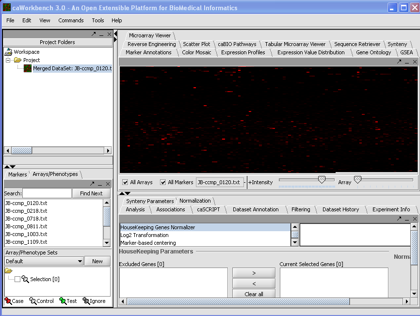
| + | Your File Nodes will now be Merged into one Project folder. | ||
| + | |||
| + | [[Image:(T)MLoadingData1.png]] | ||
| + | |||
| + | '''''<u>To Merge Data From Experiments Already Loaded</u>''''' | ||
| + | |||
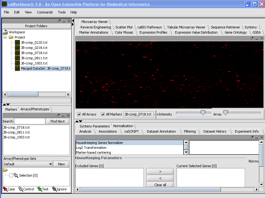
| + | '''1.''' Select the Project Nodes that you want to Merge. | ||
| + | |||
| + | '''2.''' Left click on file, choose Merge Datasets. | ||
| + | |||
| + | [[Image:(T)MFileScreen1.png]] | ||
| + | |||
| + | |||
| + | '''<u>You Can Rename a Project and/or a Project Node</u>''' | ||
| + | |||
| + | |||
| + | '''<u>''Renaming A Project''</u>''' | ||
| + | |||
| + | '''1.''' Right mouse click on Project folder. | ||
| + | |||
| + | '''2.''' Select Rename. | ||
| + | |||
| + | [[Image:(T)MReNameProject.png]] | ||
| + | |||
| + | '''3.''' In Pop-up Screen Rename your Project. | ||
| + | |||
| + | '''4.''' Click on the '''Okay''' button | ||
| + | |||
| + | |||
| + | '''<u>''Renaming a Project Node''</u>''' | ||
| + | |||
| + | '''1.''' Right mouse click on Project Node. | ||
| + | |||
| + | '''2.''' Select Rename. | ||
| + | |||
| + | [[Image:(T)MReNameProjectNode.png]] | ||
| + | |||
| + | '''3.''' In Pop-up Screen Rename your Project Node. | ||
| + | |||
| + | '''4.''' Click on the '''Okay''' button. | ||
| + | |||
| + | |||
| + | |||
| + | |||
| + | '''<u>You Can Remove a Project and/or a Project Node</u>''' | ||
| + | |||
| + | |||
| + | '''<u>''Removing A Project''</u>''' | ||
| + | |||
| + | '''1.''' Right mouse click on Project folder. | ||
| + | |||
| + | '''2.''' Select Remove. | ||
| + | |||
| + | '''3.''' You will no longer see the Project folder. | ||
| + | |||
| + | |||
| + | '''<u>''Removing a Project Node''</u>''' | ||
| + | |||
| + | '''1.''' Right mouse click on Project Node. | ||
| + | |||
| + | '''2.''' Select Remove Project. | ||
| + | |||
| + | '''3.''' You will no longer see the Project Node. | ||
| + | |||
| + | |||
| + | '''<u>''Saving a File 'Node'</u>''' | ||
| + | |||
| + | '''1.''' Right mouse click on File(s) 'Node(s)' that you want to save. | ||
| + | |||
| + | '''2.''' Click on the Save.''' | ||
| + | |||
| + | |||
| + | [[Image:(T)MSavingAFile.png]] | ||
| + | |||
| + | The Save Screen will come up. | ||
| + | |||
| + | [[Image:(T)MSavingAFile1.png]] | ||
| + | |||
| + | '''3.''' Choose a location. | ||
| + | |||
| + | '''4.''' Name your File(s) 'Node(s)' | ||
| + | |||
| + | '''5.''' Click on the '''Save''' button | ||
| + | |||
| + | |||
| + | '''<u>Load, Add, and/or Modify Remote Data</u>''' | ||
| + | |||
| + | There will be times that you may need data from a Remote Location, with this program you are able to load, add, and/or modify that data. | ||
| + | |||
| + | When the File Screen comes up click on the Remote Radial button and you will see this screen. | ||
| + | The Open File Dialog Window is updated so that you can work with your Remote Sources. | ||
| + | |||
| + | [[Image:(T)MEditRemoteData.png]] | ||
| + | |||
| + | The four buttons on the bottom of this screen are what you will be working with | ||
| + | |||
| + | '''''Basic Usage''''' | ||
| + | |||
| + | '''caArray''' button - Gives you a listing of your Remote Resources. | ||
| + | |||
| + | '''Go''' button - Accesses the Remote Source that you selected. | ||
| + | |||
| + | '''Add A New Resource''' button - Opens the Data Source Definition Page used to add Remote Data. | ||
| + | |||
| + | '''Edit''' button - Edits Remote Source Parameters. | ||
| + | |||
| + | |||
| + | '''''To Add A Remote Source''''' | ||
| + | |||
| + | '''1.''' Click on the '''Add A New Resource''' button. | ||
| + | |||
| + | [[Image:(T)MRemoteData2.png]] | ||
| + | This is the Data Source Definition Page | ||
| + | |||
| + | '''2.''' Fill in the Data Source definition page. URL and Short Name are required fields. | ||
| + | |||
| + | '''3.''' Click on the OK button. | ||
| + | |||
| + | The configuration is set up to automatically reflect your additional Data Source. | ||
| + | |||
| + | |||
| + | '''''To Modify A Remote Source''''' | ||
| + | |||
| + | '''1.''' Select the File that you want to modify. | ||
| + | |||
| + | [[Image:(T)MRemoteData1.1.png]] | ||
| + | |||
| + | '''2.''' Click on the '''Edit''' button. | ||
| + | |||
| + | |||
| + | [[Image:(T)MRemoteData3.png]] | ||
| + | |||
| + | '''3.''' Make the changes that you need. | ||
| + | |||
| + | '''4.''' Click on the '''OK''' button | ||
| + | |||
| + | End Mary:::::::::::::: | ||
| + | |||
| + | |||
| + | |||
| + | ===Loading Data=== | ||
| + | |||
| + | When first started, geWorkbench appears so: | ||
| + | |||
| + | [[Image:T_StartupState.png]] | ||
| + | |||
| + | |||
| + | Right-click on the '''Workspace''' entry in the '''Project Folders''' window at upper left to create a new project. | ||
| + | |||
| + | [[Image:T_NewProject.png]] | ||
| + | |||
| + | |||
| + | |||
| + | Next, right-click on the new project entry and select '''Open Files'''. | ||
| + | |||
| + | [[Image:T_OpenFiles.png]] | ||
| + | |||
| + | |||
| + | |||
| + | Here we will select 10 MAS5 format text files from the directory geworkbench\data\training\cardiogenomics.med.harvard.edu, which is included in the geWorkbench download: | ||
| + | |||
| + | [[Image:T_SelectMAS5.png]] | ||
| + | |||
| + | |||
| + | |||
| + | The chip type HG_U95Av2 is recognized... | ||
| + | |||
| + | [[Image:T_Chip_type_message.png]] | ||
| + | |||
| + | |||
| + | |||
| + | The read-in data is displayed in the '''Microarray Panel'''. Note we have increased the instensity slider to maximum here. | ||
| + | |||
| + | [[Image:T_MAS5_display.png]] | ||
| + | |||
| + | |||
| + | |||
| + | We can now assign phenotypes to each chip. We will place the phenotypes in the default group, however you can create new phenotype groups by pushing the '''New''' button on the '''Phenotype Panel''' at lower left. | ||
| + | |||
| + | Here we select and label arrays in the '''Phenotype Panel''' which contain samples from the congestive cardiomyopathy disease state... | ||
| + | |||
| + | [[Image:T_PanelLabelCardio.png]] | ||
| + | |||
| + | |||
| + | |||
| + | Next, we can similarly label the remaining arrays as "Normal". We have also checked boxes to indicate that these groups of arrays are "Active". Various analysis and visualization components can be set to only use/display activated arrays or markers. | ||
| + | |||
| + | [[Image:T_PhenotypesPriorToCase.png]] | ||
| + | |||
| + | |||
| + | |||
| + | For statistical tests such as the t-test the Case and Control groups can be specified. This is done by left-clicking on the thumb-tack icon in front of the phenotype name. Here we are specifying the disease arrays as the "Case". The remaining "Normal" arrays are by default labeled control. | ||
| + | [[Image:T_PhenotypeSettingCase.png]] | ||
| + | |||
| + | |||
| + | |||
| + | A red thumbtack indicates the arrays have been specified as "Case". | ||
| + | |||
| + | [[Image:T_PhenotypeCaseSet.png]] | ||
| + | |||
| + | |||
| + | |||
| + | We can also rename the merged dataset by clicking on its entry in the '''Project Panel'''. | ||
| + | |||
| + | [[Image:T_RenameDataset.png]] | ||
| + | |||
| + | |||
| + | |||
| + | Here we will call it CCMP. | ||
| + | |||
| + | [[Image:T_RenamingDataset.png]] | ||
| + | |||
| + | |||
| + | |||
| + | With the datasets merged, classified and named, we can save the dataset for future use. We will call it "cardiomyopathy.exp" (.exp is the default extension for the geWorkbench matrix file type). | ||
| + | |||
| + | [[Image:T_SaveProject.png]] | ||
| + | |||
| + | |||
| + | |||
| + | The default display of microarray data is an absolute display. We can change it to a relative display by selecting Tools:Preferences from the top menubar. We have removed the dataset so that we can read it back in using the new preferences. | ||
| + | |||
| + | [[Image:T_ChangePrefs.png]] | ||
| + | |||
| + | |||
| + | |||
| + | Here we select the '''relative''' display type. | ||
| + | |||
| + | [[Image:T_ChangePrefsToRelative.png]] | ||
| + | |||
| + | |||
| + | |||
| + | Returning to the Open File dialog as we before by right-clicking on the project entry, we will select the "cardiomyopathy.exp" file we previously saved... | ||
| + | |||
| + | [[Image:T_OpenCardio.png]] | ||
| + | |||
| + | |||
| + | |||
| + | Resulting in the following colorful display of the array data for the first array.... | ||
| + | |||
| + | [[Image:T_RelativeDisplay.png]] | ||
| + | |||
| + | |||
| + | |||
| + | |||
| + | |||
[[Image:(T)MarGettingStarted.png]] | [[Image:(T)MarGettingStarted.png]] | ||
Revision as of 20:22, 27 February 2006
Outline
In this tutorial, you will learn how to:
- Create a new Project.
- Load microarray data.
- Merge data from several loaded microarray experiments.
- Rename a project and/or project node.
- Remove a project and/or project node.
- Save project files that you have created.
- Load, add, and/or modify remote data.
Supported data formats
- Microarray
- Affymetrix MAS5/GCOS Files.This one will be used for the tutorial. brief explanation of file type needed
- Affymetrix File Matrix - this is the native file type created by geWorkbench.
- RMA Express File - RMA Express is a sophisticated tool for combining data from multiple Affymetrix chips.
- Affy Excel or txt data file.
- Normalized no-confidence expression matrix. A variant of the geWorkbench file matrix format that omits the confidence value columns (P-value or Present/Absent calls).
- Genepix Files - An analysis program for two color arrays.
- Other
- FASTA Files. DNA or protein sequence files in FASTA format.
- Pattern Files.
- Genotypic data Files.
Workspaces and Projects
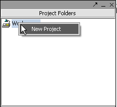
1.To create a New Project, right-click on Workspace in the Project Folders area at upper left.
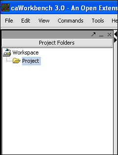
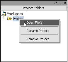
2. Left-click on Project.
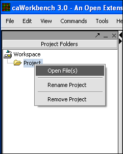
3. a new Project folder will be created. right-click on it, then left-click on open files.
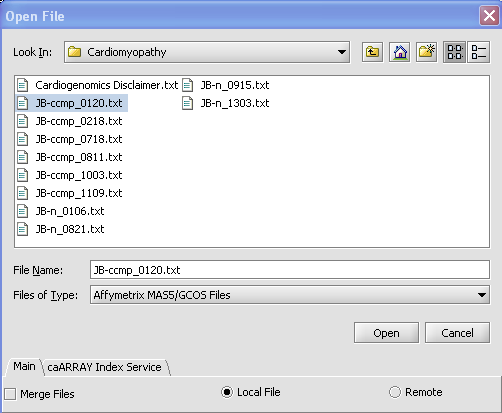
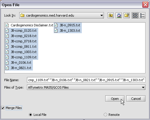
4. Find the type of file that you want to work with. In this case it will be Affymetrix MAS5/GCOS Files.
5. Find the file that you want to work with and select.
6. Make sure Local radio button is selected.
7. Click on the Open button.
Your File is now loaded:
You Can Merge Data From Several Loaded Microarray Experiments Into One Project Folder
Different Microarray files can be merged so that they can be viewed and analyzed together. As long as files are of the same type you can merge them into one project node. You can do this during the original loading process, or after you have already loaded a file.
To Merge Data From The Original Loading Process
1. Right mouse click on the Project folder.
2. Select the files that you want to Merge.
3. Select the Merge Files box.
4. Left mouse click on the Open button.
Your File Nodes will now be Merged into one Project folder.
To Merge Data From Experiments Already Loaded
1. Select the Project Nodes that you want to Merge.
2. Left click on file, choose Merge Datasets.
You Can Rename a Project and/or a Project Node
Renaming A Project
1. Right mouse click on Project folder.
2. Select Rename.
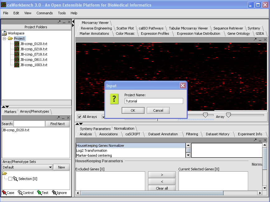
3. In Pop-up Screen Rename your Project.
4. Click on the Okay button
Renaming a Project Node
1. Right mouse click on Project Node.
2. Select Rename.
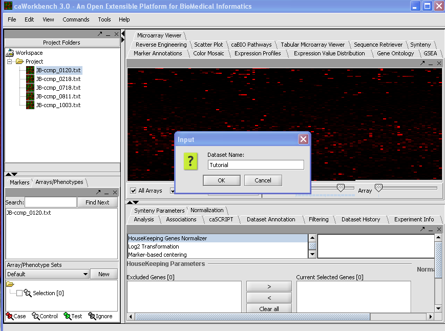
3. In Pop-up Screen Rename your Project Node.
4. Click on the Okay button.
You Can Remove a Project and/or a Project Node
Removing A Project
1. Right mouse click on Project folder.
2. Select Remove.
3. You will no longer see the Project folder.
Removing a Project Node
1. Right mouse click on Project Node.
2. Select Remove Project.
3. You will no longer see the Project Node.
Saving a File 'Node'
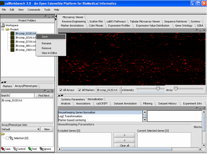
1. Right mouse click on File(s) 'Node(s)' that you want to save.
2. Click on the Save.
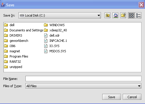
The Save Screen will come up.
3. Choose a location.
4. Name your File(s) 'Node(s)'
5. Click on the Save button
Load, Add, and/or Modify Remote Data
There will be times that you may need data from a Remote Location, with this program you are able to load, add, and/or modify that data.
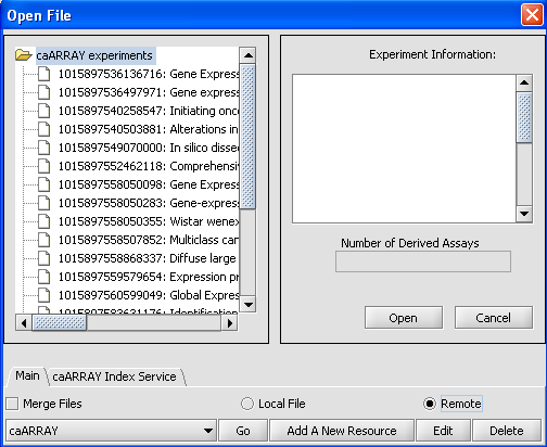
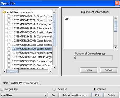
When the File Screen comes up click on the Remote Radial button and you will see this screen. The Open File Dialog Window is updated so that you can work with your Remote Sources.
The four buttons on the bottom of this screen are what you will be working with
Basic Usage
caArray button - Gives you a listing of your Remote Resources.
Go button - Accesses the Remote Source that you selected.
Add A New Resource button - Opens the Data Source Definition Page used to add Remote Data.
Edit button - Edits Remote Source Parameters.
To Add A Remote Source
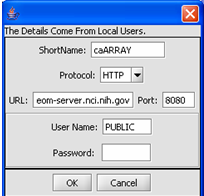
1. Click on the Add A New Resource button.
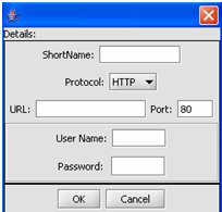 This is the Data Source Definition Page
2. Fill in the Data Source definition page. URL and Short Name are required fields.
3. Click on the OK button.
The configuration is set up to automatically reflect your additional Data Source.
To Modify A Remote Source
1. Select the File that you want to modify.
2. Click on the Edit button.
3. Make the changes that you need.
4. Click on the OK button
End Mary::::::::::::::
Loading Data
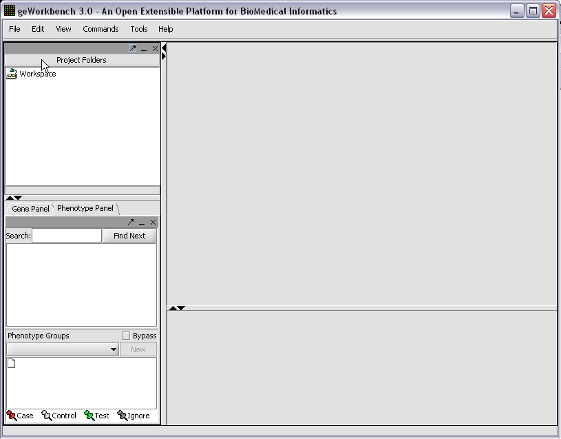
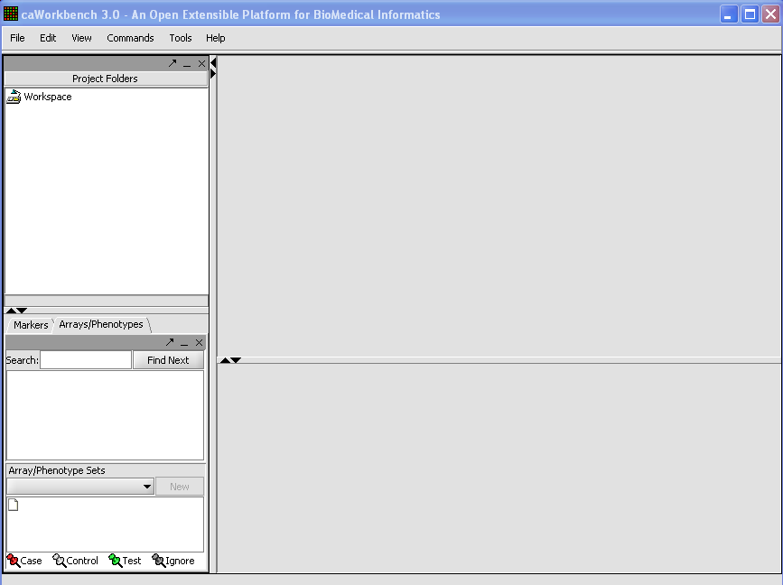
When first started, geWorkbench appears so:
Right-click on the Workspace entry in the Project Folders window at upper left to create a new project.
Next, right-click on the new project entry and select Open Files.
Here we will select 10 MAS5 format text files from the directory geworkbench\data\training\cardiogenomics.med.harvard.edu, which is included in the geWorkbench download:
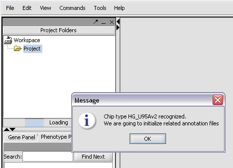
The chip type HG_U95Av2 is recognized...
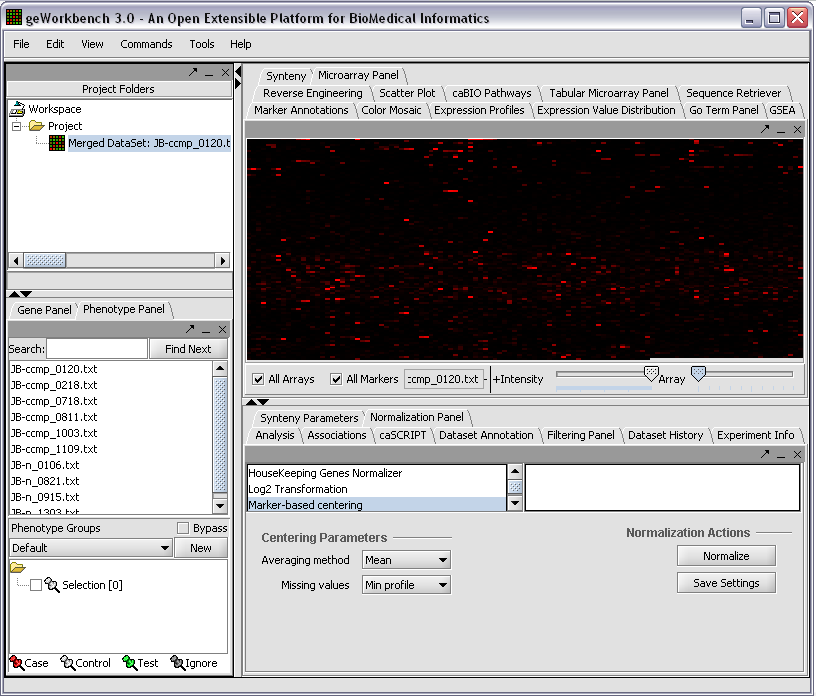
The read-in data is displayed in the Microarray Panel. Note we have increased the instensity slider to maximum here.
We can now assign phenotypes to each chip. We will place the phenotypes in the default group, however you can create new phenotype groups by pushing the New button on the Phenotype Panel at lower left.
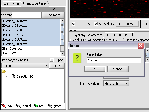
Here we select and label arrays in the Phenotype Panel which contain samples from the congestive cardiomyopathy disease state...
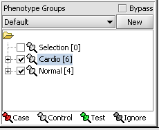
Next, we can similarly label the remaining arrays as "Normal". We have also checked boxes to indicate that these groups of arrays are "Active". Various analysis and visualization components can be set to only use/display activated arrays or markers.
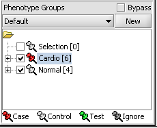
For statistical tests such as the t-test the Case and Control groups can be specified. This is done by left-clicking on the thumb-tack icon in front of the phenotype name. Here we are specifying the disease arrays as the "Case". The remaining "Normal" arrays are by default labeled control.
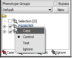
A red thumbtack indicates the arrays have been specified as "Case".
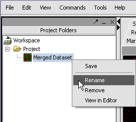
We can also rename the merged dataset by clicking on its entry in the Project Panel.
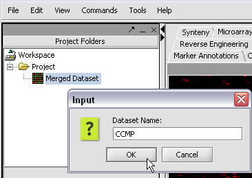
Here we will call it CCMP.
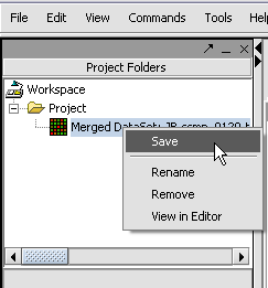
With the datasets merged, classified and named, we can save the dataset for future use. We will call it "cardiomyopathy.exp" (.exp is the default extension for the geWorkbench matrix file type).
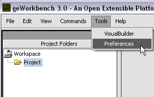
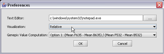
The default display of microarray data is an absolute display. We can change it to a relative display by selecting Tools:Preferences from the top menubar. We have removed the dataset so that we can read it back in using the new preferences.
Here we select the relative display type.
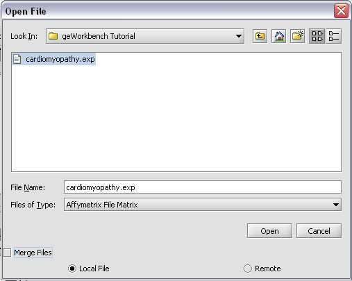
Returning to the Open File dialog as we before by right-clicking on the project entry, we will select the "cardiomyopathy.exp" file we previously saved...
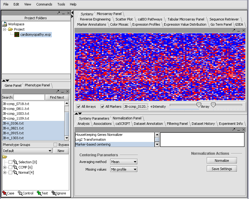
Resulting in the following colorful display of the array data for the first array....
