Revision as of 16:48, 27 February 2006

The tutorials shown on this page provide a quick introduction to the most important features of geWorkbench. Additional information can be found in the User Guide (in preparation) and in the Online Help section of the program.

Getting Started

Obtaining and installing geWorkbench. Requirements.

Overview

A brief introduction to the use of geWorkbench.

Loading and Saving Data

Loading microarray data files, merging into one dataset, and saving.

Data Subsets

Subsets of both markers and arrays can be defined for targeted analysis.

Viewing a Microarray Dataset

Survey of geWorkbench visusaliztion tools for microarray data.

Filtering and Normalizing

geWorkbench provides numerous methods for filtering and normalizing microarray data.

Differential Expression

Several variants of the t-test are available.

Clustering

Data can be clustered using a fast hierarchical clustering routine, as well as SOMs.

Marker Annotations

Marker annotations can be retrieved, including BioCarta pathway diagrams.

Sequence Retrieval

Genomic sequences for markers can be retrieved for further analysis.

Pattern Discovery

Upstream seqeunce can be analyzed for conserved sequence patterns.

Promoter Analysis

Search a set of sequences against a promoter database.

Reverse Engineering

Microarray datasets can be analyzed for interactions between markers.

GO Term Enrichment

Determine if particluar Gene Ontology terms are overrepresented in a data subset.

BLAST

geWorkbench can run BLAST jobs on the JCSB cluster.

Synteny

Compare genomic sequence from two different species.

(NOTE: This section of our web site is under active development. More tutorials are forthcoming, covering many usage scenarios for geWorkbench.)

Getting Started

With geWorkbench you can work with both mircoarray gene expression data and with gene or protein sequences. Many kinds of analysis are supported - for microarrays, there are filtering and normalization, basic statistical analyses, clustering, network reverse engineering, as well as many common visualization tools. For sequence data there are routines such as BLAST, pattern detection, transcription factor mapping, and syntenic region analyis. Furthermore, genomic sequences around markers of interest found in microarray experiements can be easily retrieved and, for example, used for promoter/TF analysis.

geWorkbench is designed from the ground up to be extensible. New modules can be programmed to interact directly with its framework, or existing code can be wrapped in a geWorkbench adaptor to allow seamless communications with the framework and other modules.

To start using geWorkbench, one must supply initial datafiles. For microarray data, several formats are currently available, including MAS5/GCOS text files, GenePix files, and a simple, geWorkbench-specific matrix format. In the next section, we will show how to read in MAS5 format files and write out a matrix file. For sequence data, fasta format files are accepted.

For the time being, the latest version of geWorkbench for Windows can be downloaded from the below link. Full download instructions and versions for Linux and Macintosh will be available in the Download section very soon. You will be offered the choice of a version with a Java Virtual Machine (JRE 1.5) included in the download (VM), and one without (NoVM).

geWorkbench3.0

Loading Data

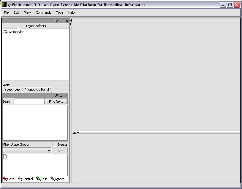
When first started, geWorkbench appears so:

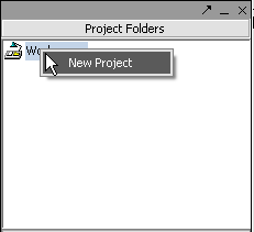
Right-click on the Workspace entry in the Project Folders window at upper left to create a new project.

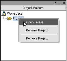
Next, right-click on the new project entry and select Open Files.

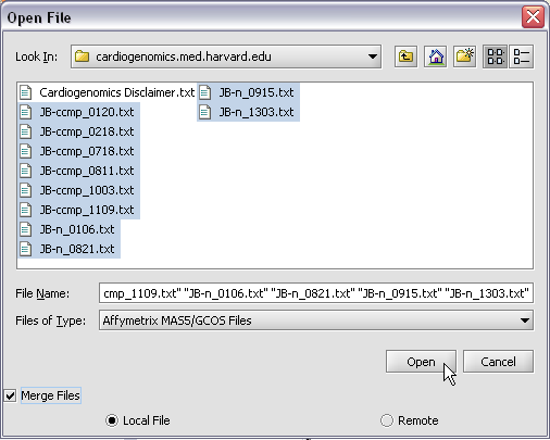
Here we will select 10 MAS5 format text files from the directory geworkbench\data\training\cardiogenomics.med.harvard.edu, which is included in the geWorkbench download:

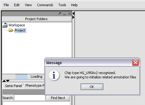
The chip type HG_U95Av2 is recognized...

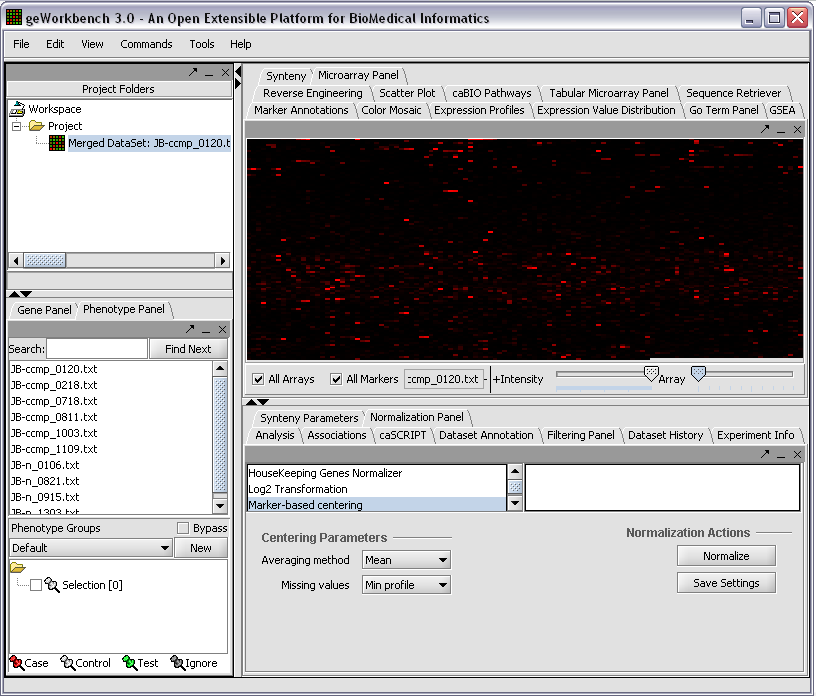
The read-in data is displayed in the Microarray Panel. Note we have increased the instensity slider to maximum here.

We can now assign phenotypes to each chip. We will place the phenotypes in the default group, however you can create new phenotype groups by pushing the New button on the Phenotype Panel at lower left.

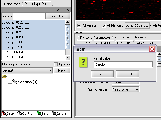
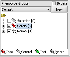
Here we select and label arrays in the Phenotype Panel which contain samples from the congestive cardiomyopathy disease state...

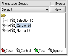
Next, we can similarly label the remaining arrays as "Normal". We have also checked boxes to indicate that these groups of arrays are "Active". Various analysis and visualization components can be set to only use/display activated arrays or markers.

For statistical tests such as the t-test the Case and Control groups can be specified. This is done by left-clicking on the thumb-tack icon in front of the phenotype name. Here we are specifying the disease arrays as the "Case". The remaining "Normal" arrays are by default labeled control.

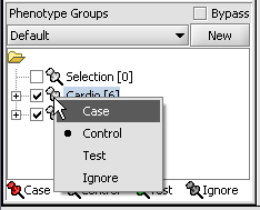
A red thumbtack indicates the arrays have been specified as "Case".

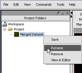
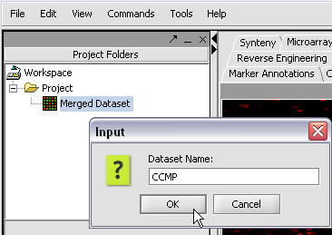
We can also rename the merged dataset by clicking on its entry in the Project Panel.

Here we will call it CCMP.

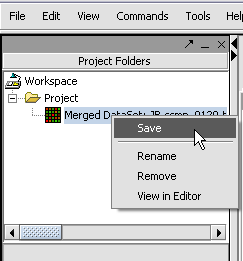
With the datasets merged, classified and named, we can save the dataset for future use. We will call it "cardiomyopathy.exp" (.exp is the default extension for the geWorkbench matrix file type).

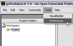
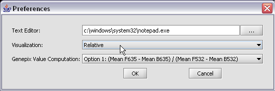
The default display of microarray data is an absolute display. We can change it to a relative display by selecting Tools:Preferences from the top menubar. We have removed the dataset so that we can read it back in using the new preferences.

Here we select the relative display type.

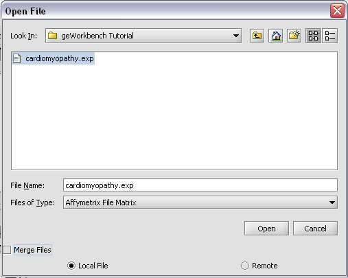
Returning to the Open File dialog as we before by right-clicking on the project entry, we will select the "cardiomyopathy.exp" file we previously saved...

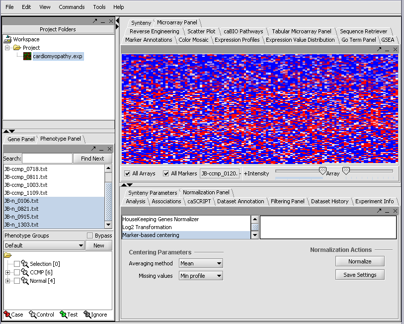
Resulting in the following colorful display of the array data for the first array....